L3 Logistic Regression. Classification. Overfitting. Regularisation.
Logistic Regression is one of the most well known regression algorithms in the world and is used extensively in classification problems (ie labelling inputs as belonging to a particular class.)
Similar principles to Linear regression apply here and we go through how we implement cost functions and gradient descent for logistic regression problems.
We also explore some new concepts. Including optimisation algorithms and some practical Matlab code implementing gradient descent, how to recognise overfitting and underfitting, and regularisation.
Logistic regression is essentially learning and forms the basis for studying Neural Nets later on.
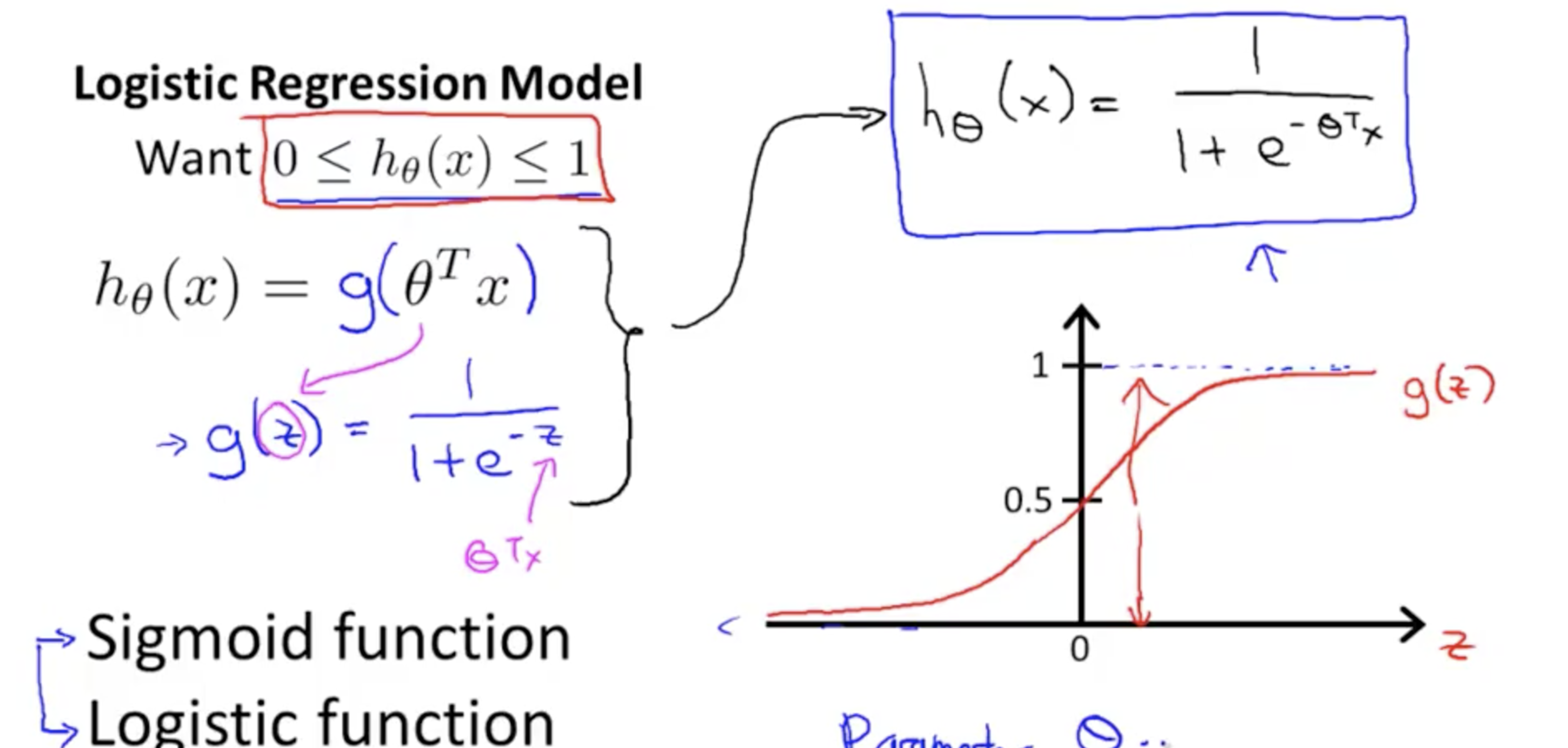
Hypothesis
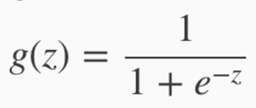
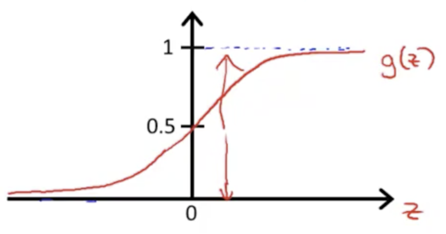
Sigmoid Function

Sigmoid function
Z = Theta Transpose * x.
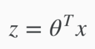
- Theta and x are vectors
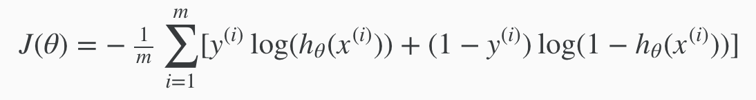
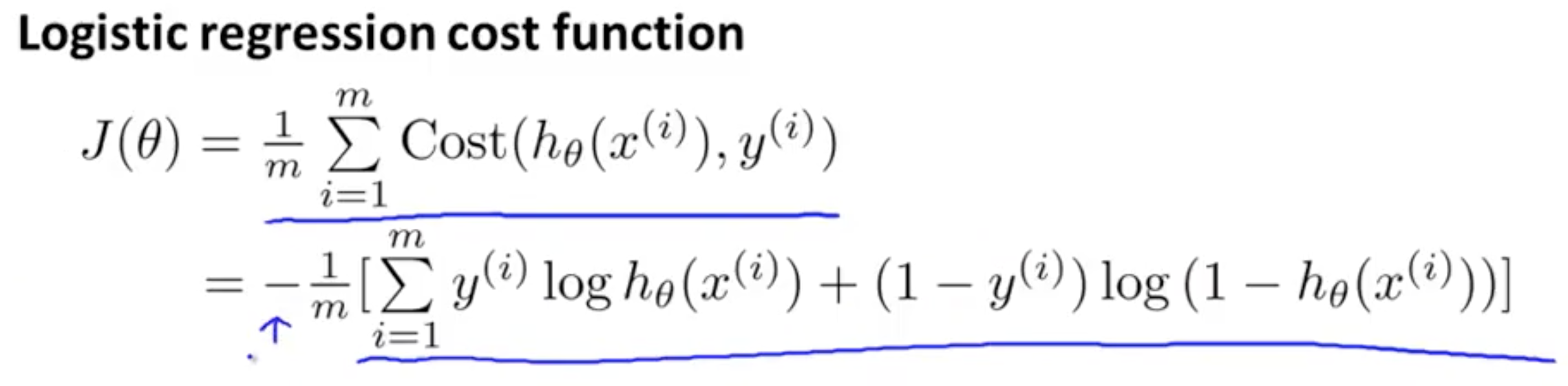
Cost Function: Regularised and Unregularised
Generalised Cost Function (for a single ith example)


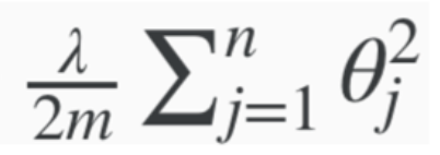
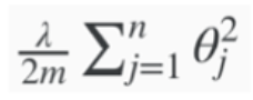
Cost Function + Regularisation

Regularised Component
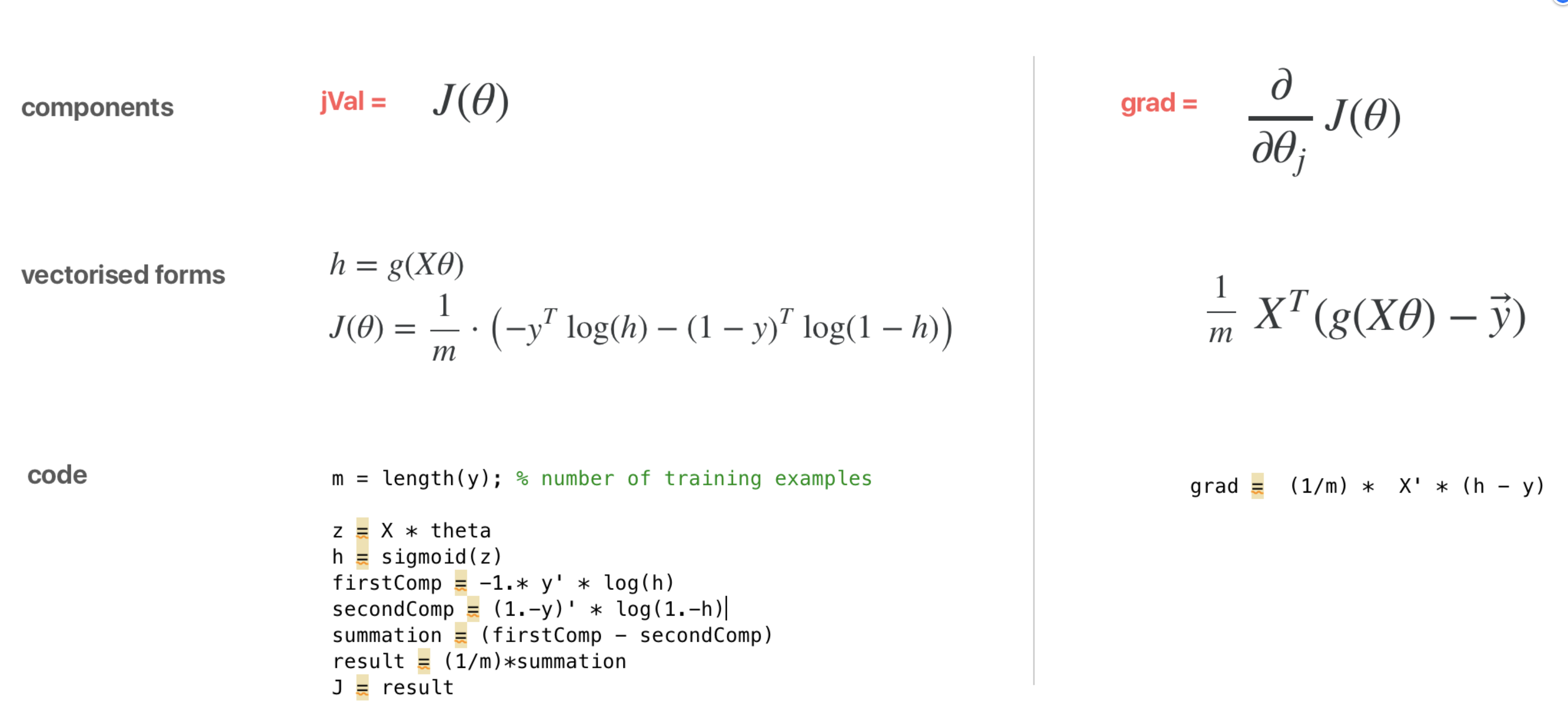
Cost Function: Vectorised
- Vectorised Unregularised Implementation (over all training examples, unregularised)
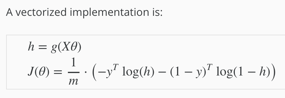
1a. In the vectorised implementation we move from looking at a single ith training example to all training examples.
1b. y and h are vectors (not matrices) covering the entire training set.
1c. So for the component 1-y, we need to subtract each training example from 1, element-wise. In matlab code this would be 1.-y
- Cost function - Regularisation Term
(Note, the regularised term for gradient descent is different to the one in the cost function)
- Now add Unregularised and Regularised Components
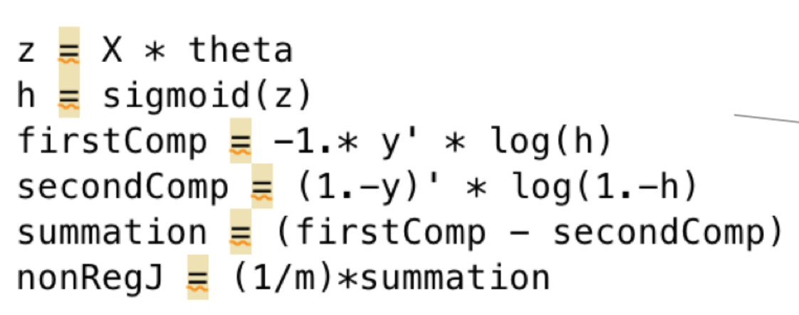
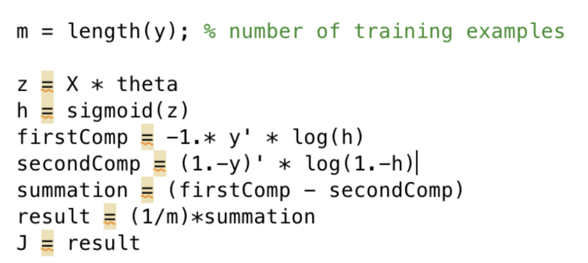
Cost Function: Code
Notice that in the code, we translate the cost function of the ith training example, to apply to the entire training set.
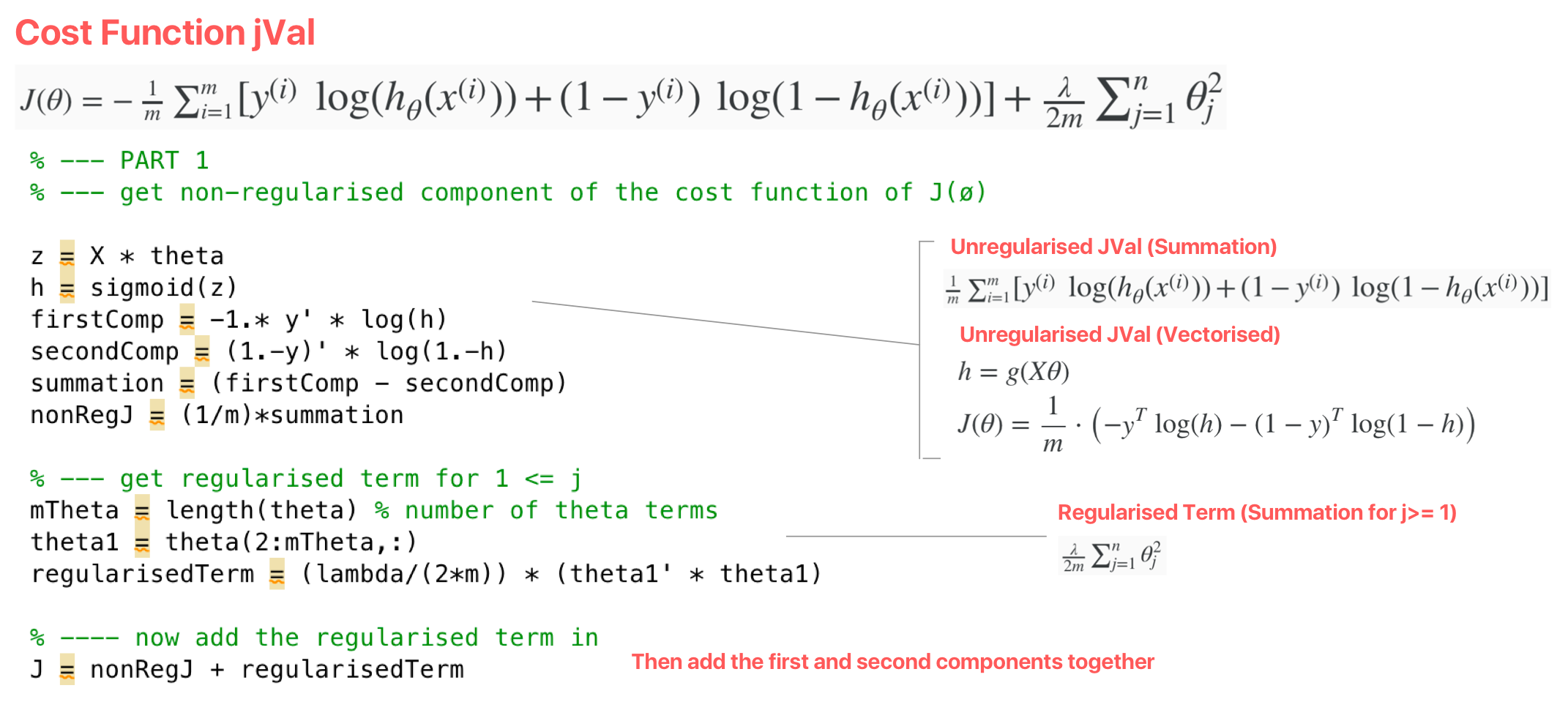
Unregularized Cost Function Component. This applies across all training examples, where h and y are matrices
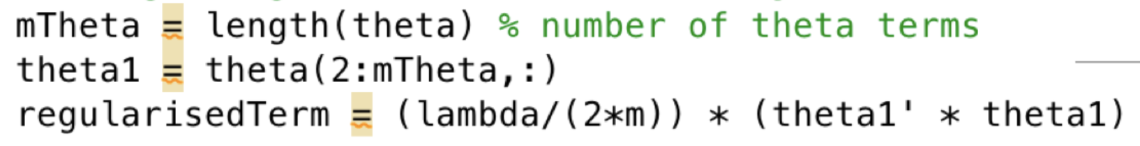
Regularisation Component. (Note: notice that theta1 squared is interpreted as Theta1' Theta1. We do this so that if theta is a m x n matrix, we can multiply so that we have a m x n n x m matrix. The transpose gets us this.)
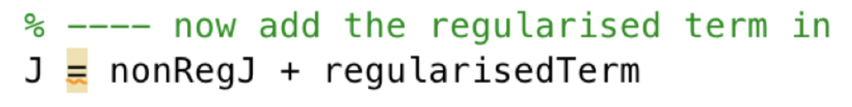
Now add Unregularised and Regularised Components
Cost Function with Regularisation. Summary + Full Code
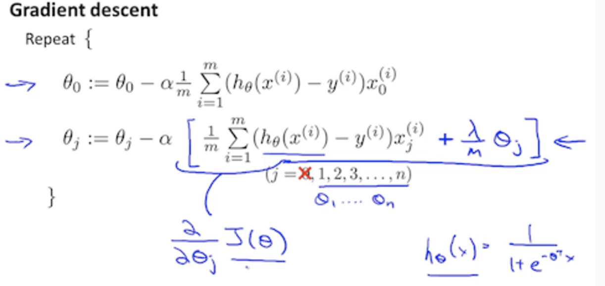
Gradient Descent
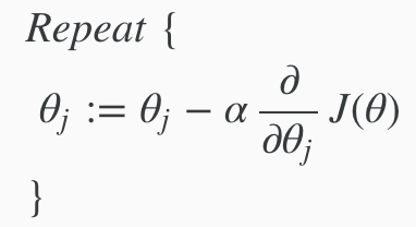
The general form for gradient decent
Gradient Descent for Cost Function for a single ith training example - It's exactly the same as the linear regression one, except that h(x) is now the Sigmoid function
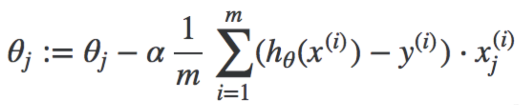
Gradient Descent. Derivative Component
Gradient Descent: Vectorised
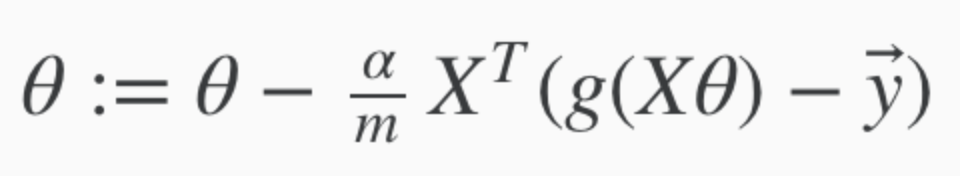
Vectorised Implementation of Gradient Descent to find min J(ø)
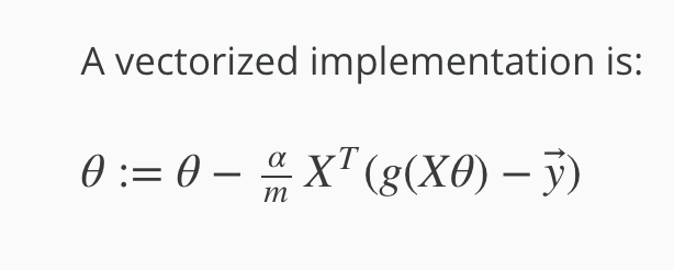
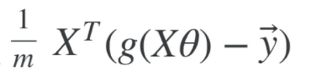
Vectorised Unregularised Component
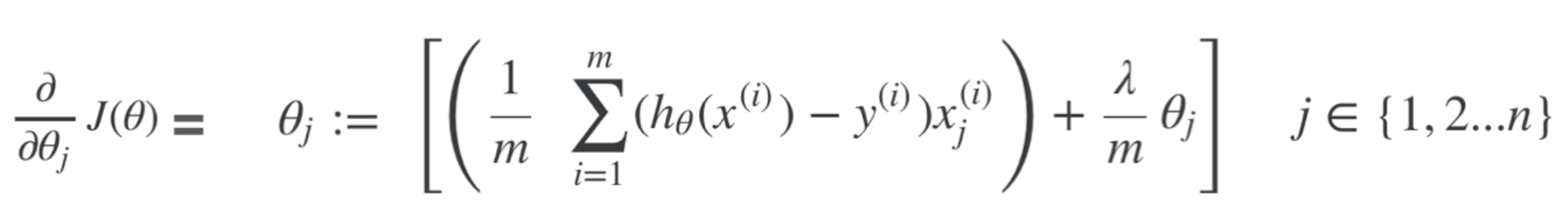
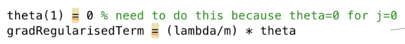
Gradient Descent - Regularisation Term
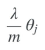
(Note, the regularised term for gradient descent is different to the one in the cost function)
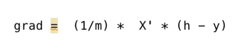
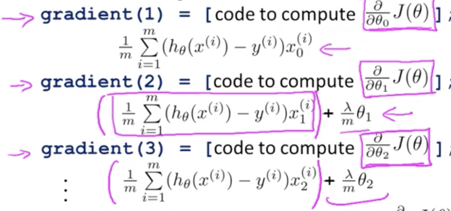
Gradient Descent: Code
Code: Gradient Descent. Overview
Code: Unregularised Gradient Descent. This applies across all training examples, where h and y are matrices
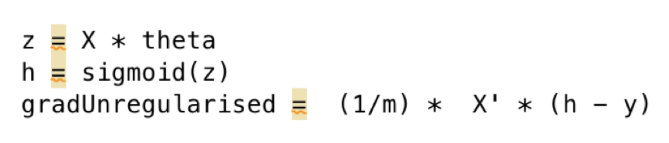
Code: Regularised Component
Now add Unregularised and Regularised Components

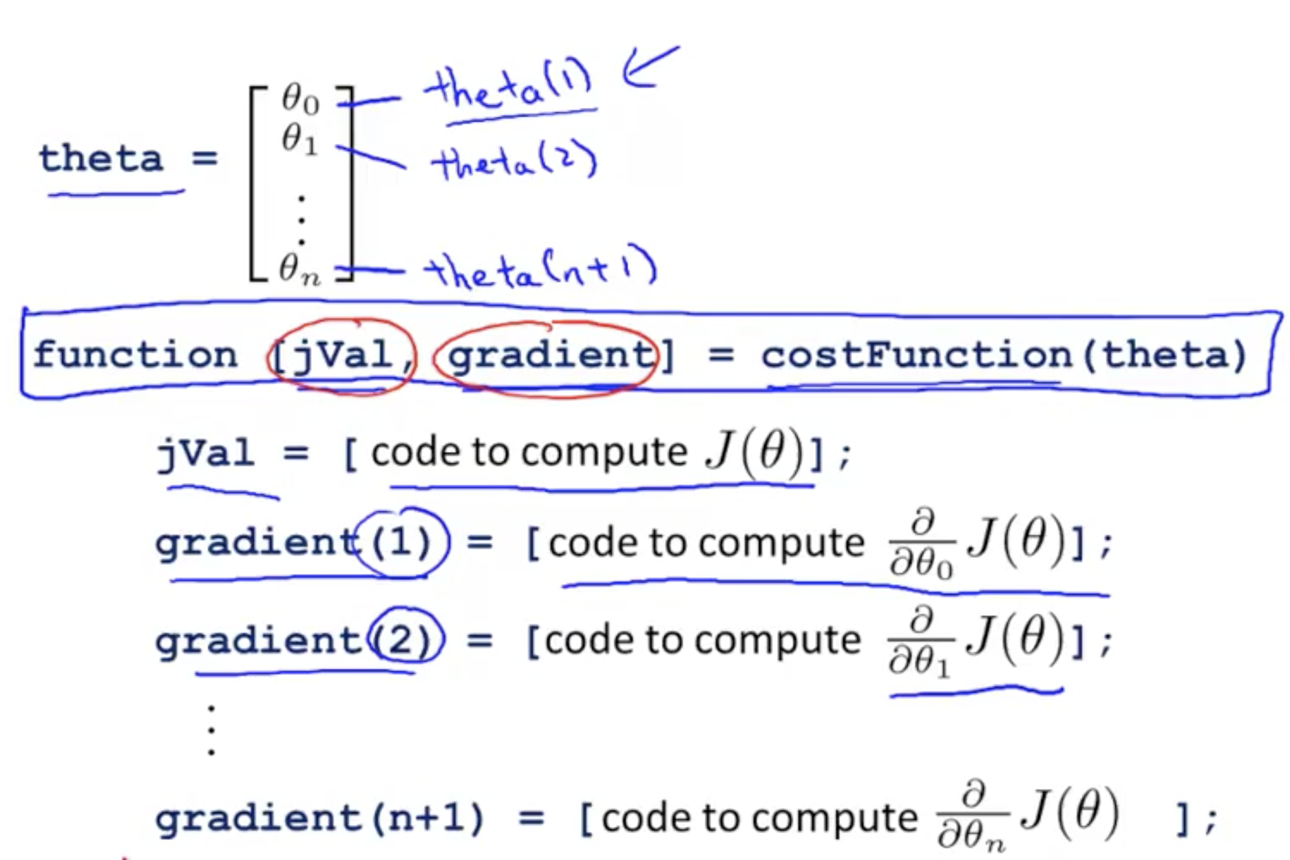
Optimiser: fminunc
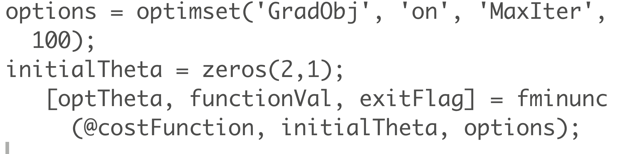
fminunc - In code we can write the following, using optimset to provide options to the fminunc function. Also, we initialise these to be a vector of zeros with dimensions that match the number of features)
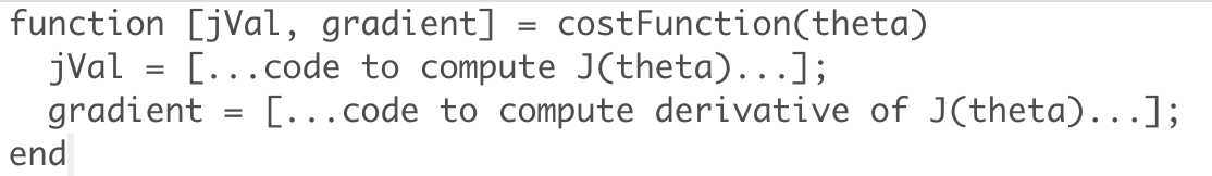
The signature of the cost function that you pass into fminunc needs to have this signature (ie return the cost value J, and the gradient, for a given theta)
fminunc let's us specify starting values for theta, and a definition of the cost function, and without choosing a value for alpha or manually looping through gradient descent, it can help us find optimal values of theta
Optimiser: fminunc code
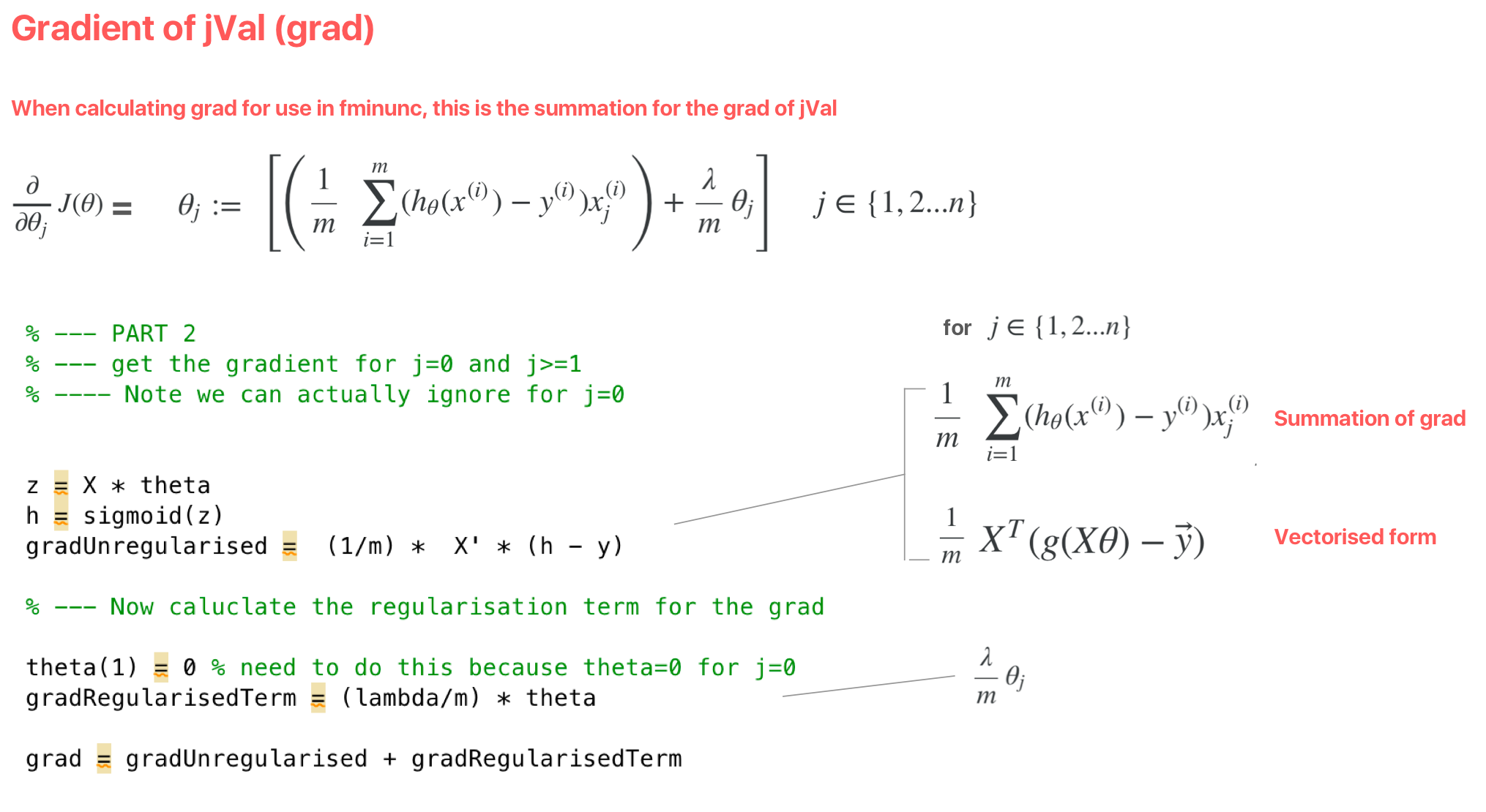
Cost function for fminunc: Calculating the cost (J) and gradient (grad) and return both in the cost function to supply to fminunc
Calculate J
Calculate grad
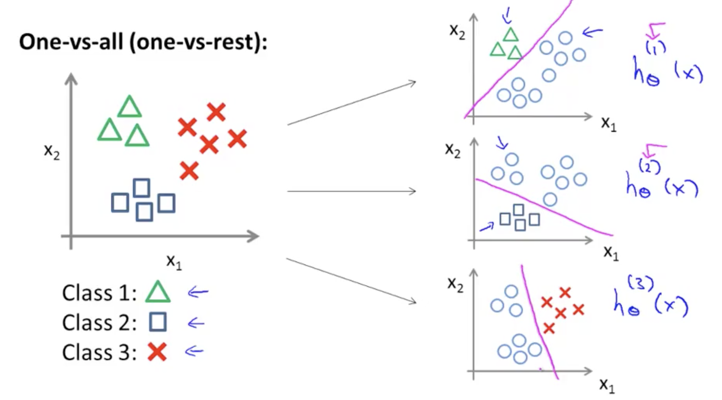
Multiclass Classification
One vs all
Gradient Descent Intuitions
"Conjugate gradient", "BFGS", and "L-BFGS" are more sophisticated, faster ways to optimize θ
Now with gradient descent
Note here that the summation doesn;t extend to the reglarised term
We first need to provide a function that evaluates the following two functions for a given input value θ:
Cost function - Intuition
Cost function - For logistic regression
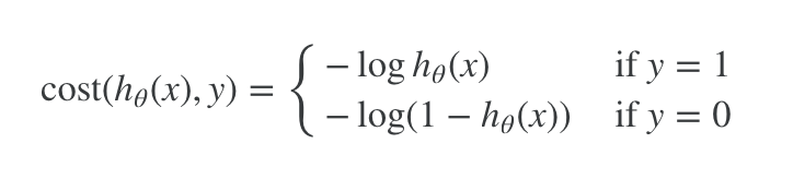
For y = 1, then the Cost function approaches infinity as h(x) decreases to 0 (ie decreases in costs because the hypothesis starts to match the actuals)
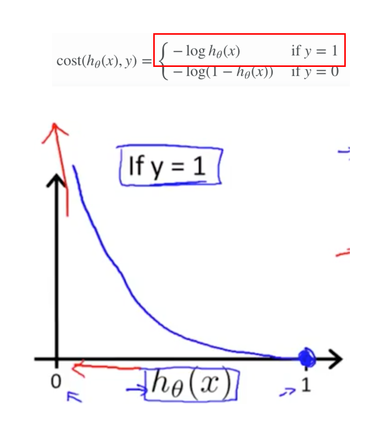
For y = 0, then the Cost function approaches infinity when h(x) increases to 1
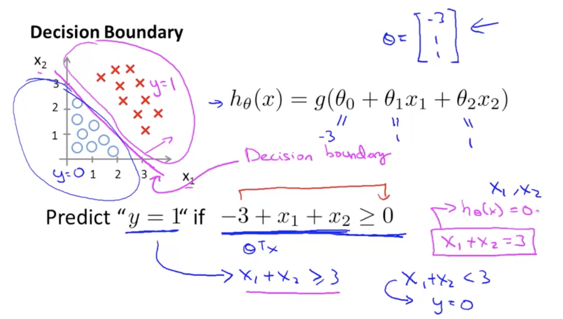
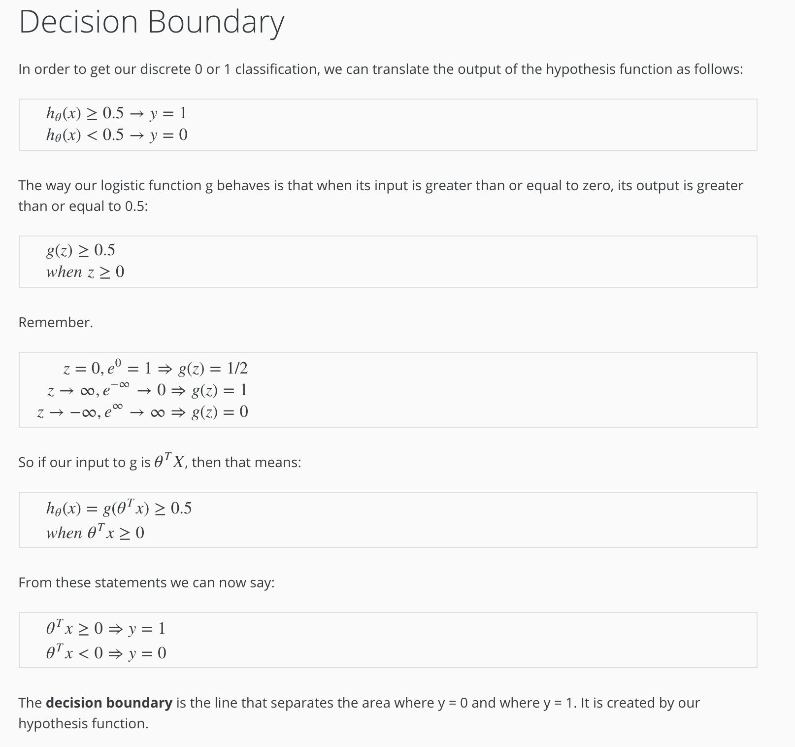
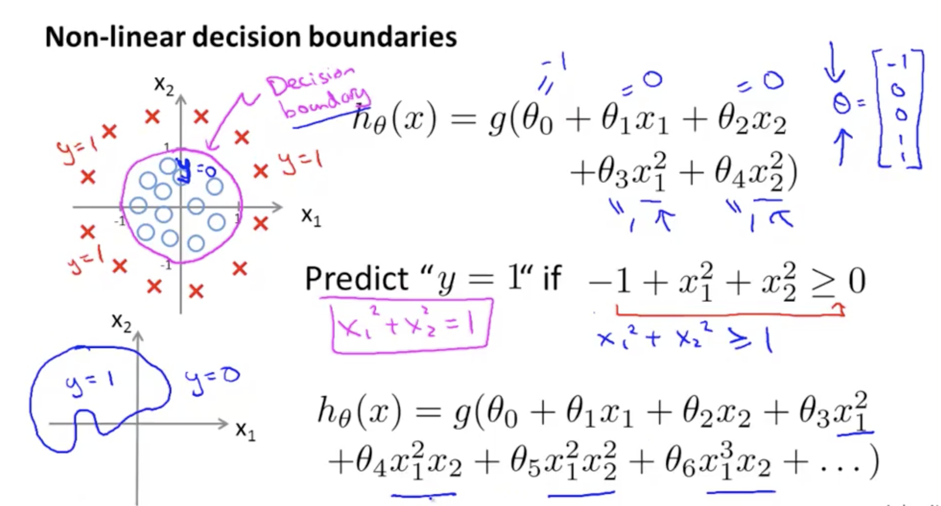
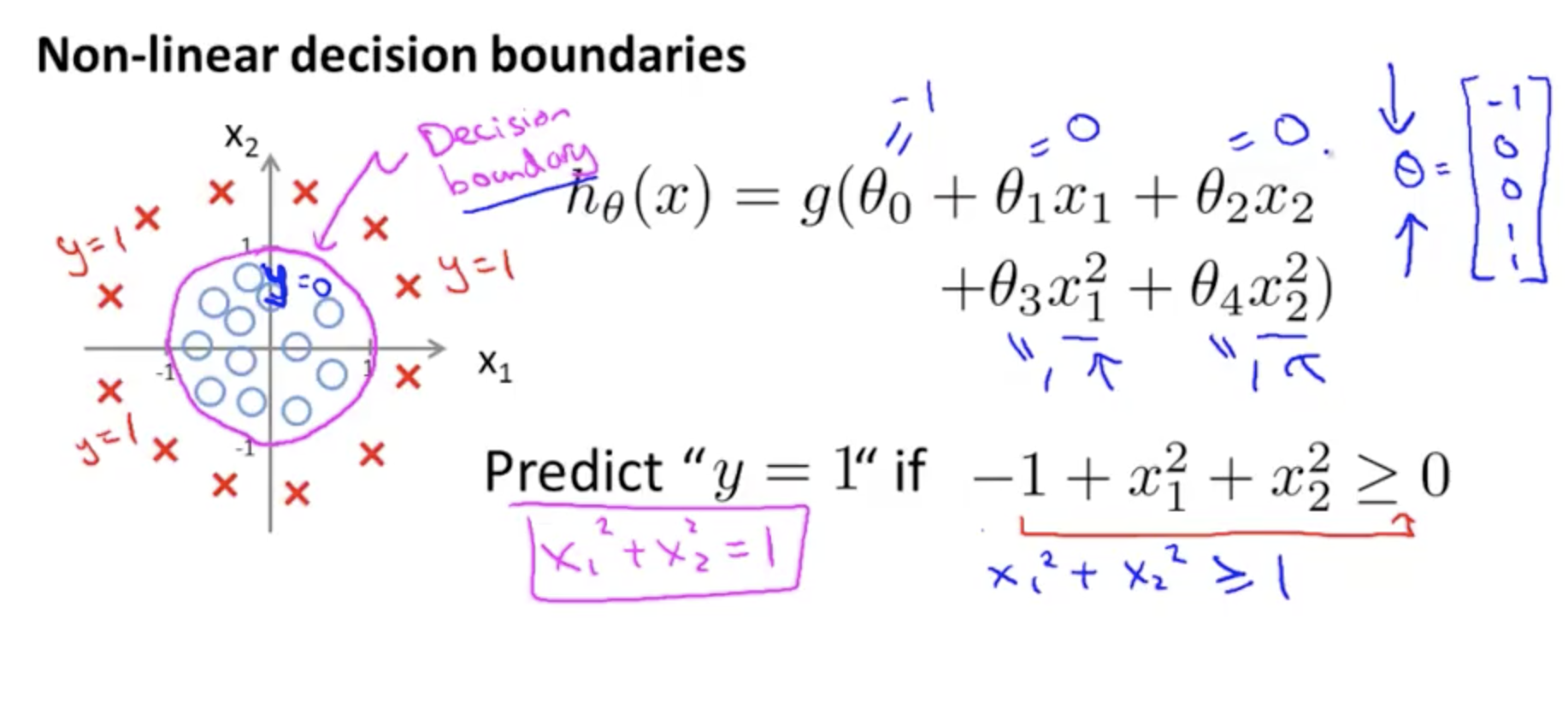
Decision Boundary
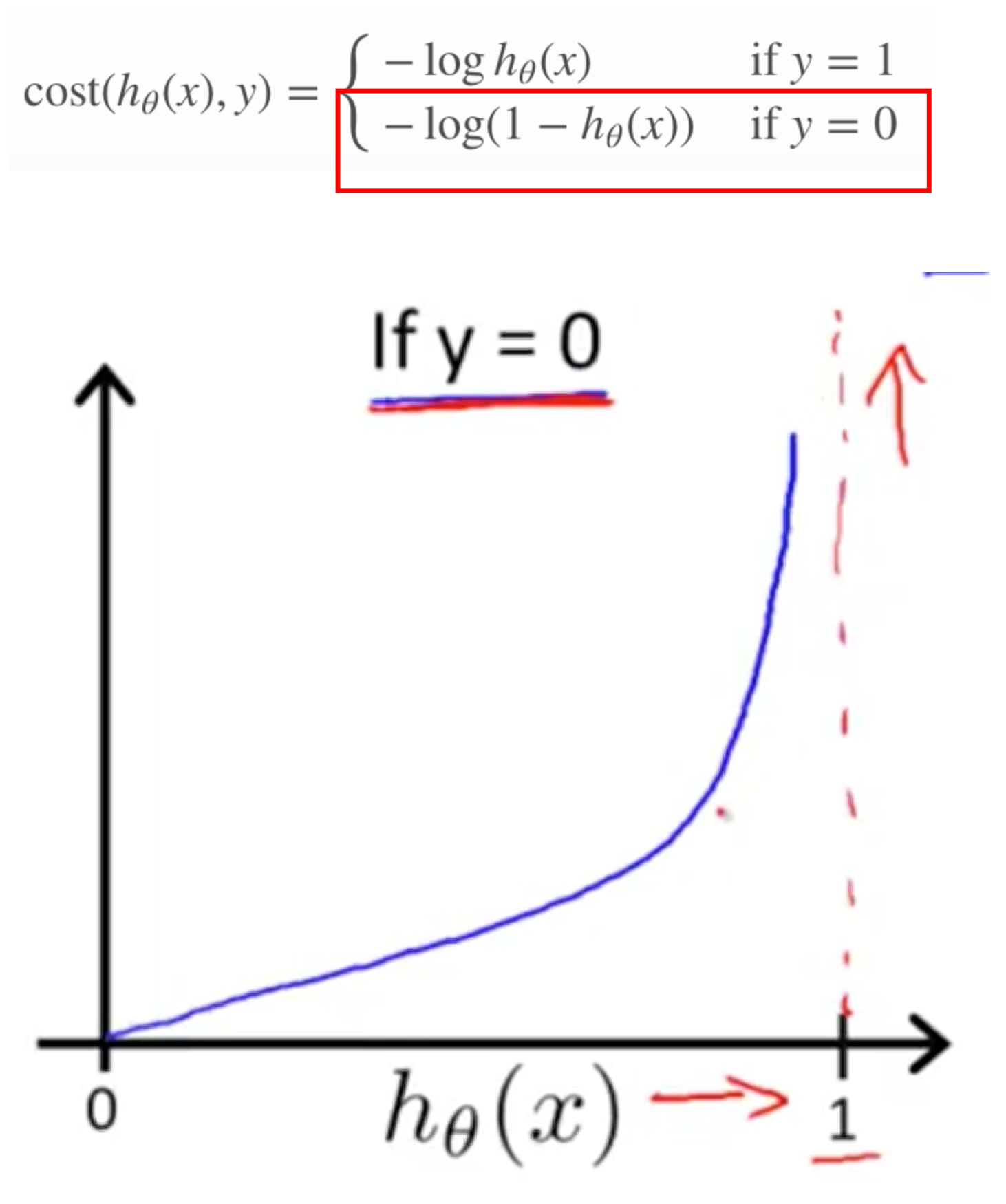
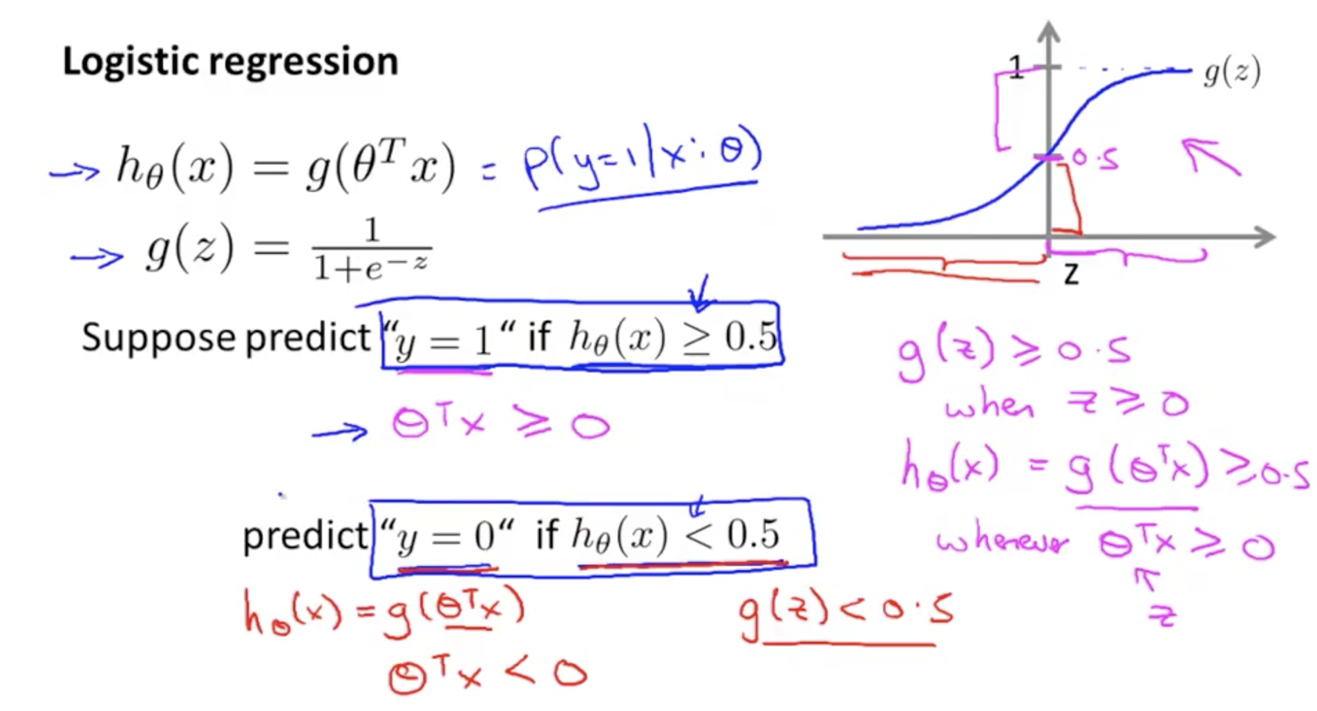
When g(z) >= 0.5, then it's INPUT (z) >= Zero

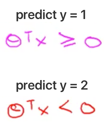
Decision Boundary - when z = ø(T)x, then when z >= 0, predicted y = 1

Decision Boundary
Summary
Non-linear decision boundaries - and choosing ø
Hypothesis Intuition
Interpretation of Sigmoid - using probabilities
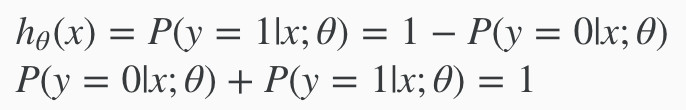
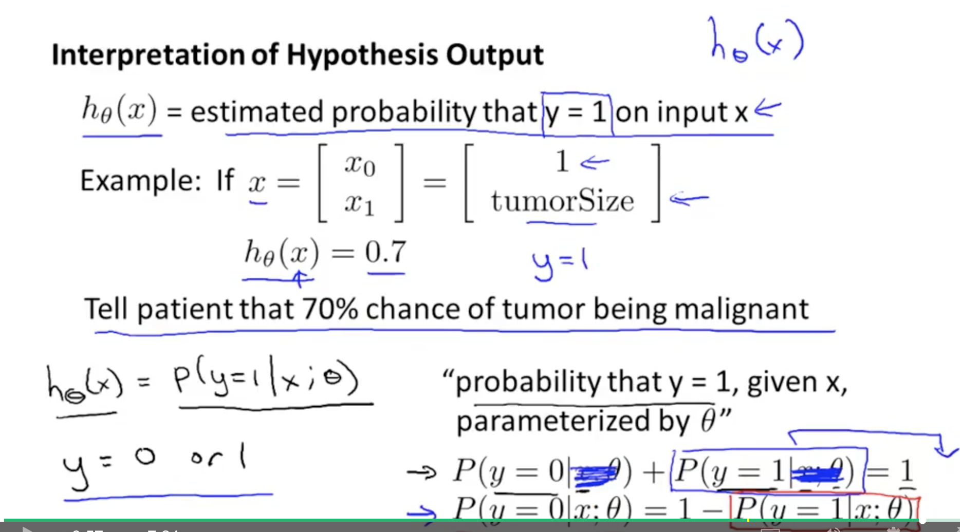
Logistic regression hypotheses function
Overfitting
Overfitting - Linear Regression
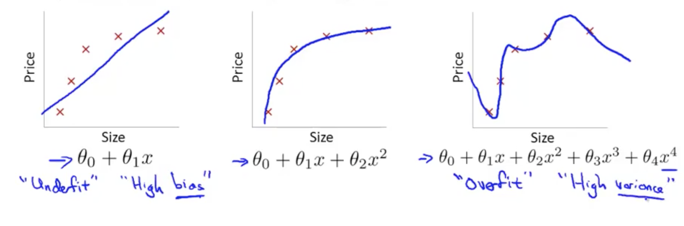
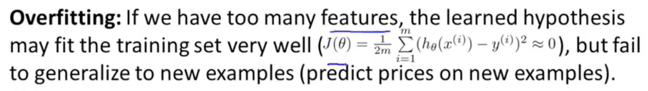
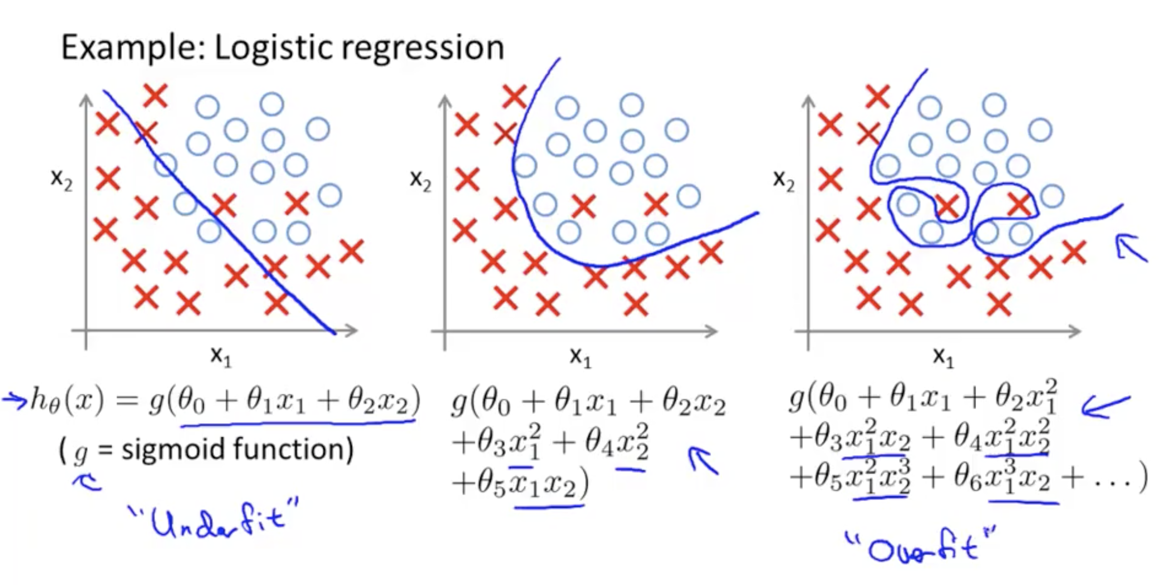
Overfitting definition - if you have too many features the learned hypothesis may fit the training set very well, but fail to generalise to new examples
Overfitting for Logisitic Regression
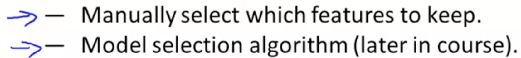
Addressing overfitting: Reduce number of features
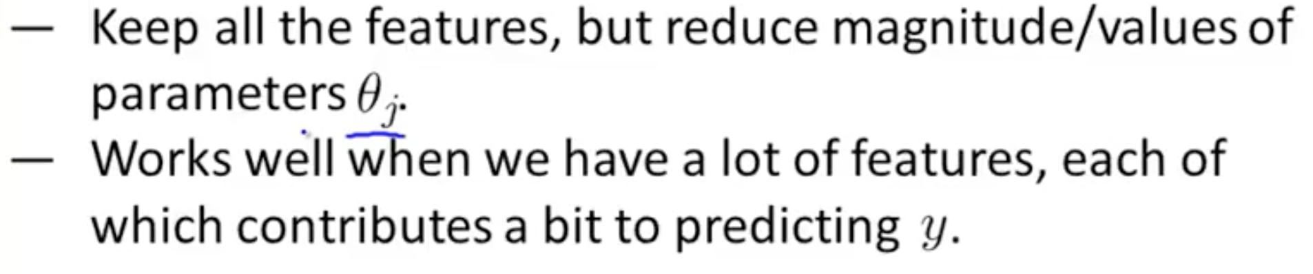
Addressing overfitting: Regularisation
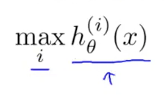
Now with all optimal h(x) computed, choose the max
Regularisation
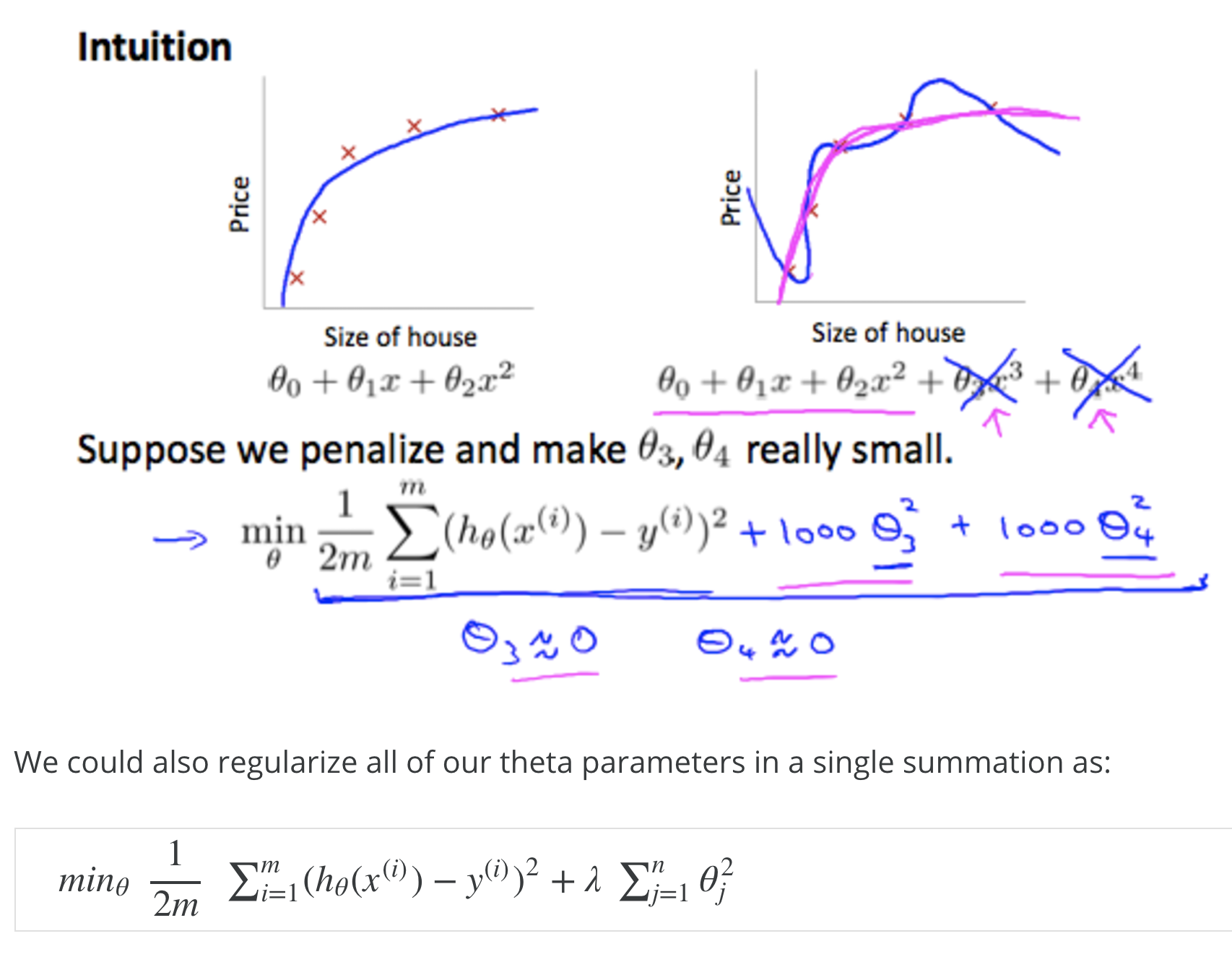
The following regularisation methods are identical for both Logistic and Linear regression. Although the examples here show linear regression, you can add the same regularisation terms to the logistic regression cost and gradient
Regularisation: Cost Function
Regularisation
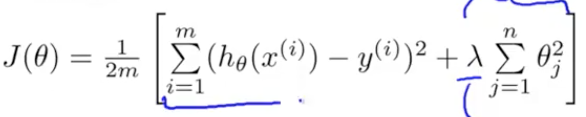
If we have overfitting from our hypothesis function h(x), we can reduce the weight that some of the terms in our function carry by INCREASING their COST in the cost function J(ø)
Don't make the regulariastaion too large, because... underfitting...
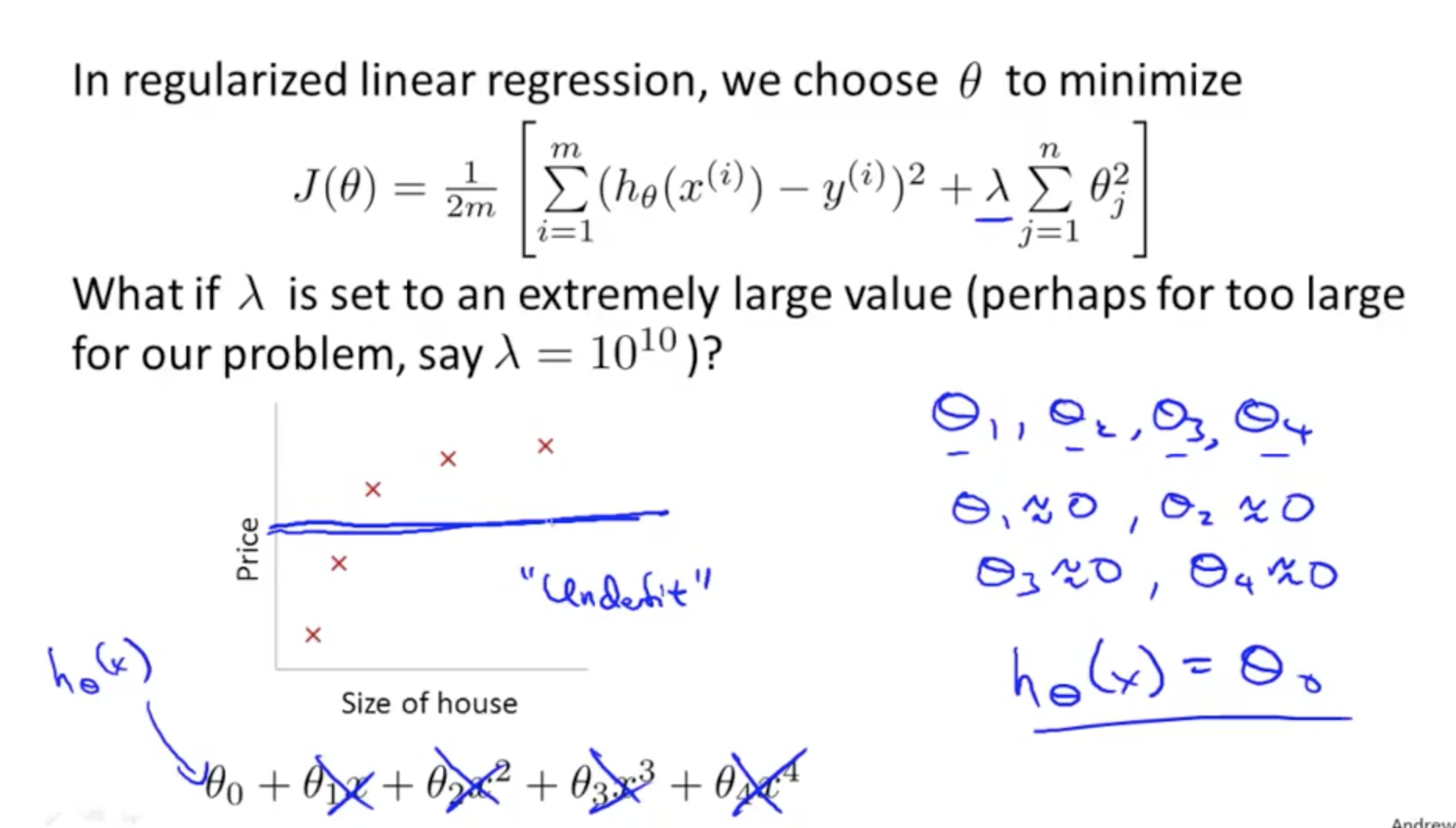
Intuition for overfitting
Regularisation: Gradient Descent
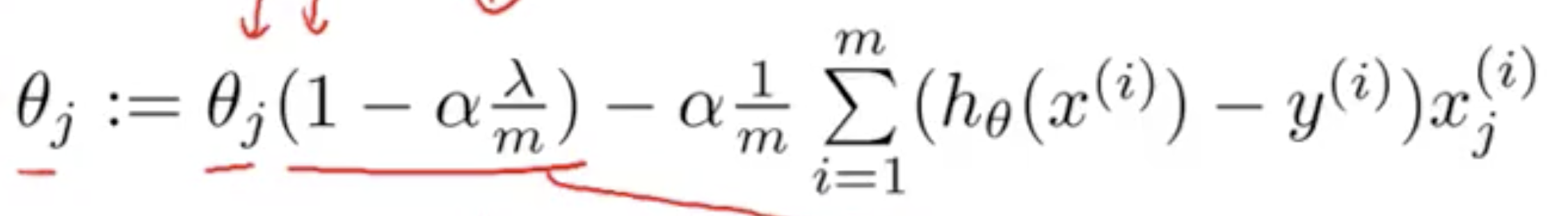
Regularisation with Gradient descent. Only add the regularisation term to theta 1 and above
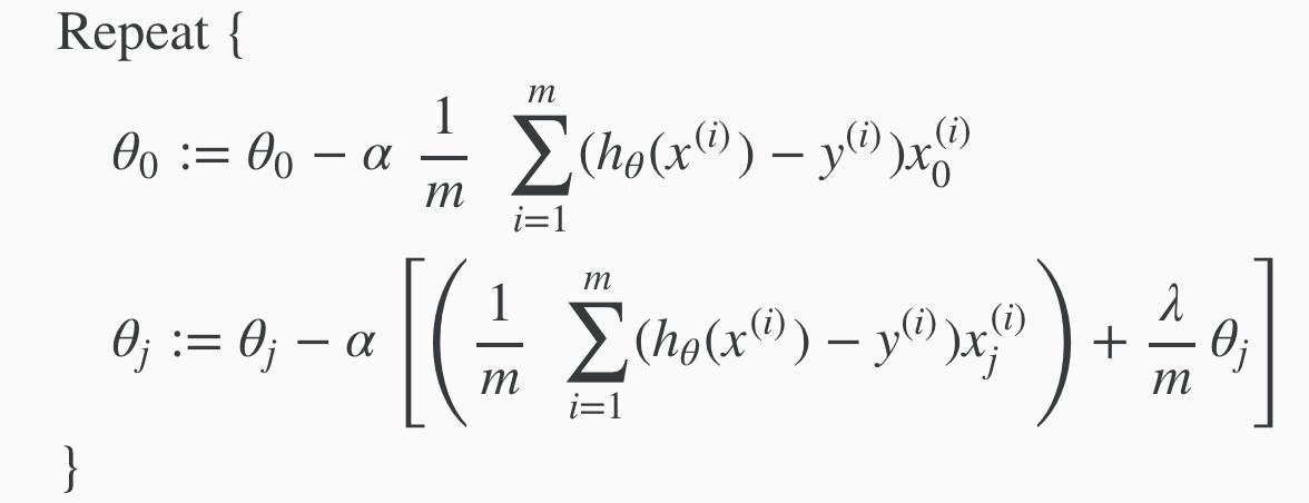
Remember: This term is outside the summation and does NOT include the bias unit. Hence why m in the summation starts from 1

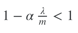
Regularisation using gradient descent can also be expressed with this.
This term in the equation above has an interesting property where it is generally less than one
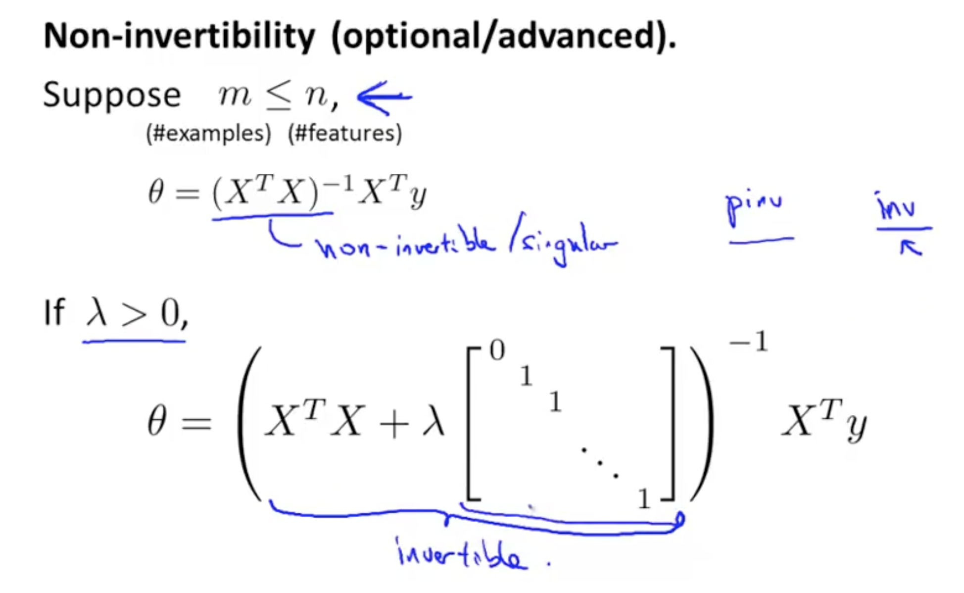
Regularisation: Normal
Regulariasation using the normal equation
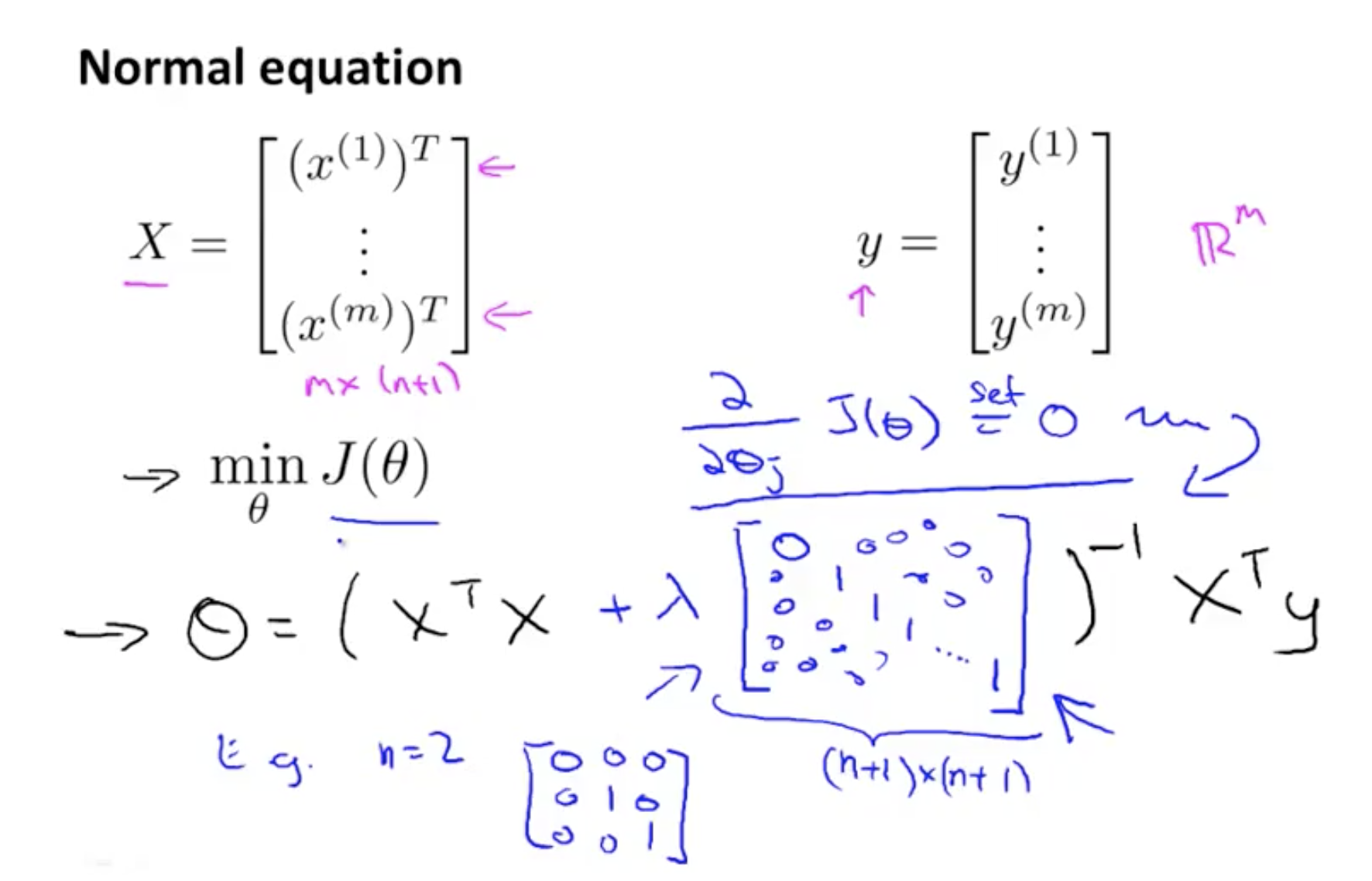
Regularisation using the normal (to find the min of J), in vector form
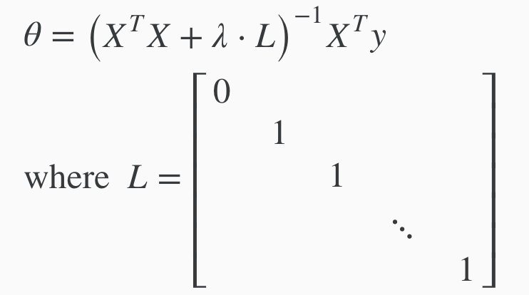
Optional (but interesting) - TLDR can avoid the problem of non-invertability by making lambda > 0. So regularisation also solves this problem if lambda is > 0