[L2] Linear Regression (Multivariate). Cost Function. Hypothesis. Gradient
In lesson 1, we were introduced to the basics of linear regression in a univariate context.
Now in lesson 2, we start to introduce models that have a number of different input features (multivariate).
We also cover the Normal equation, mean normalisation, and feature scaling.
Multivariate Hypothesis. One training example
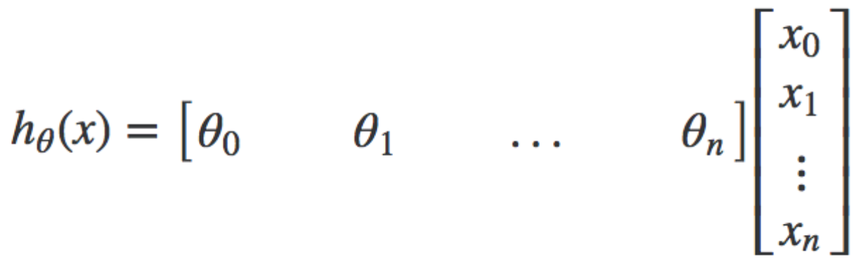
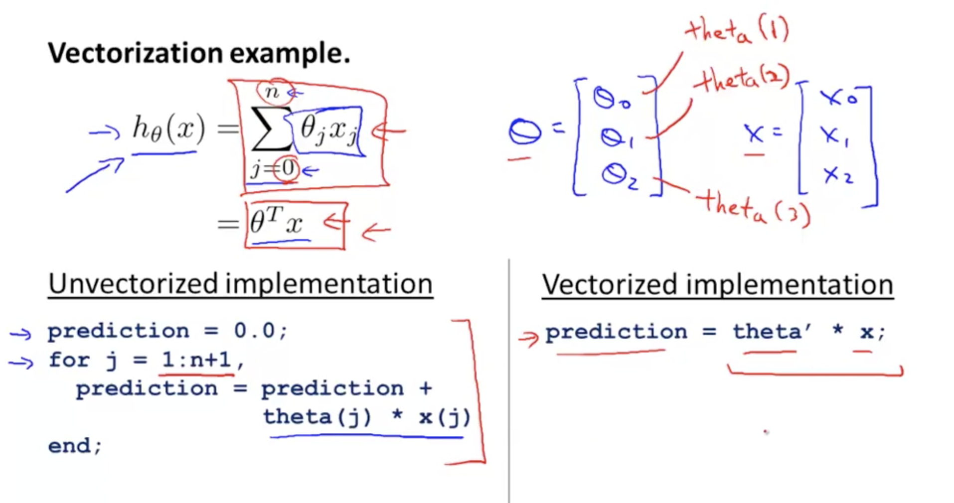
For multivariate linear regression, the hypothesis is this, for one training example. We now have multiple x features, and multiple theta weights.

We can convert this hypothesis into matrix form by doing this. Note that this is for ONE training example.
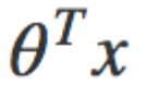
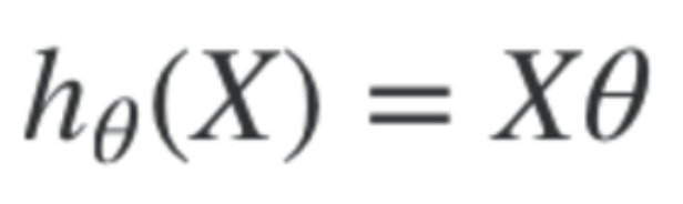
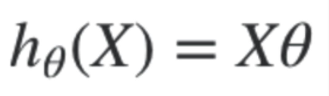
The above is more concisely expressed in this vectorised formula for the hypothesis
Additional Notes.
Summary of the info in the previous list
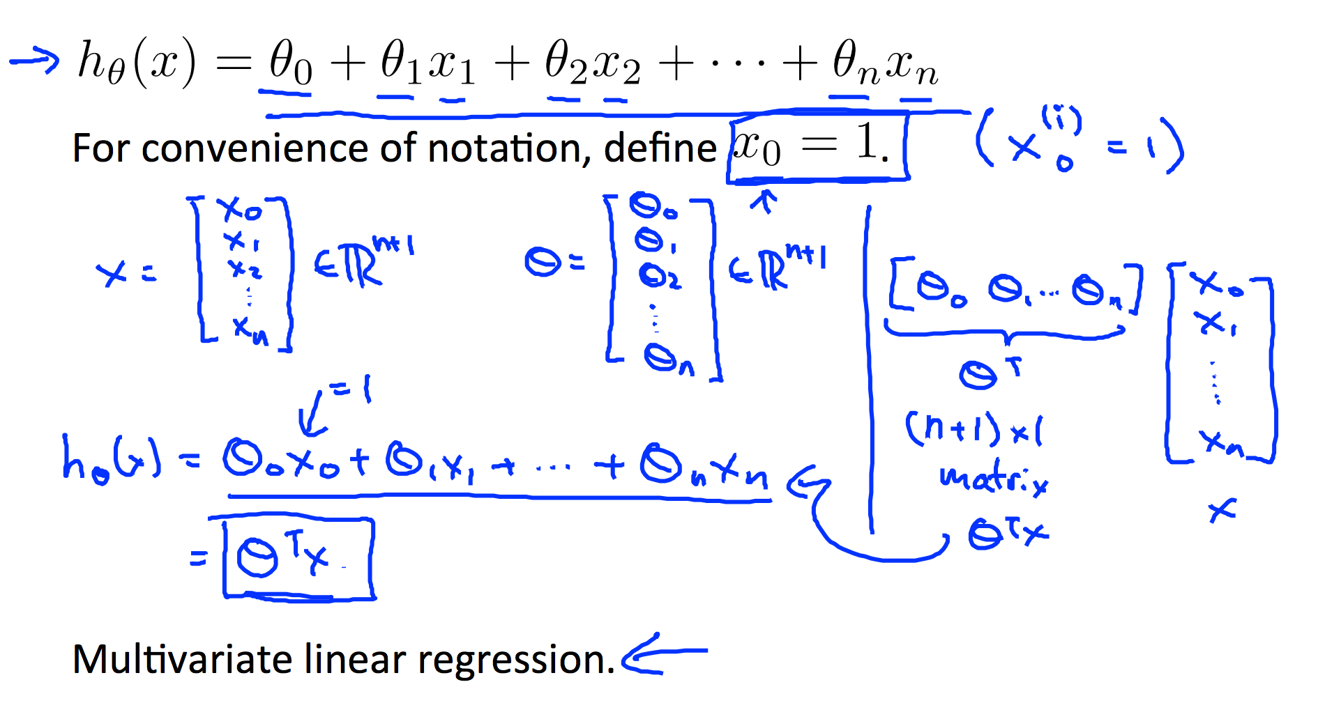
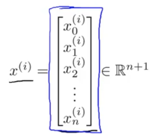
Notice that there is no x(0) term. For convenience we assume x{0}=1 with a weight of 0, so that we can use matrix multiplication
Vectorised Hypothesis
Hypothesis - Multiple training examples
With multiple training examples, we use this vectorised formula
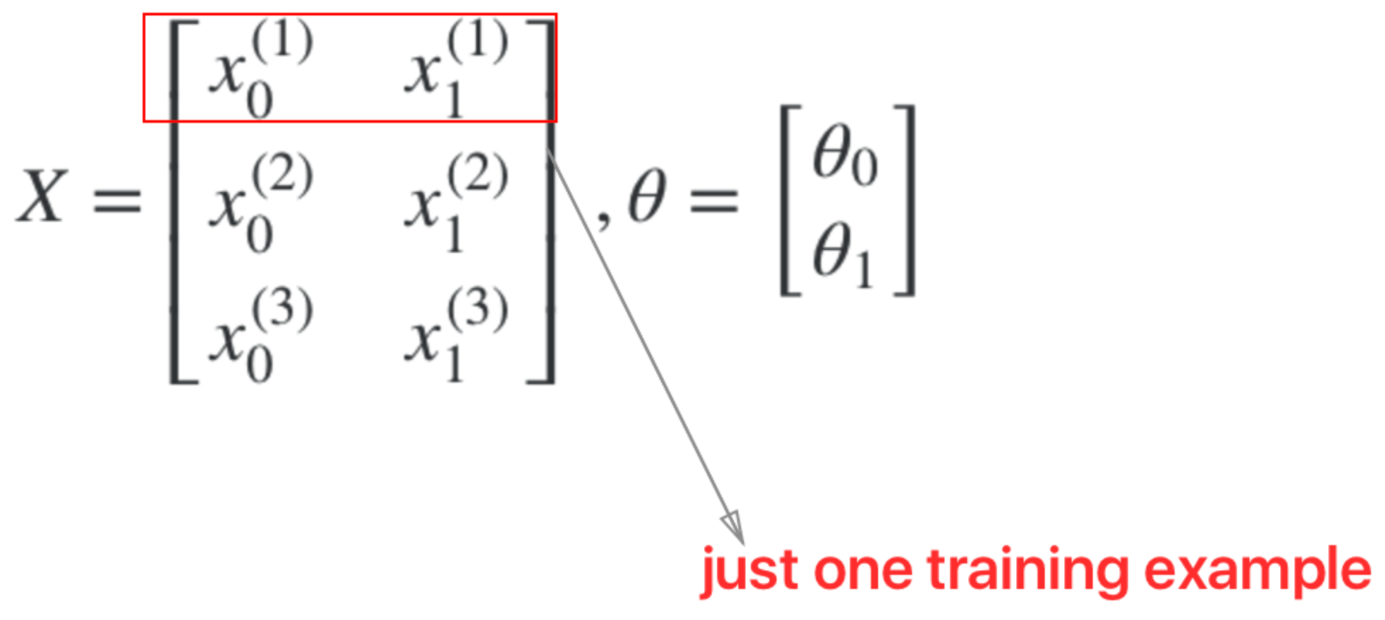
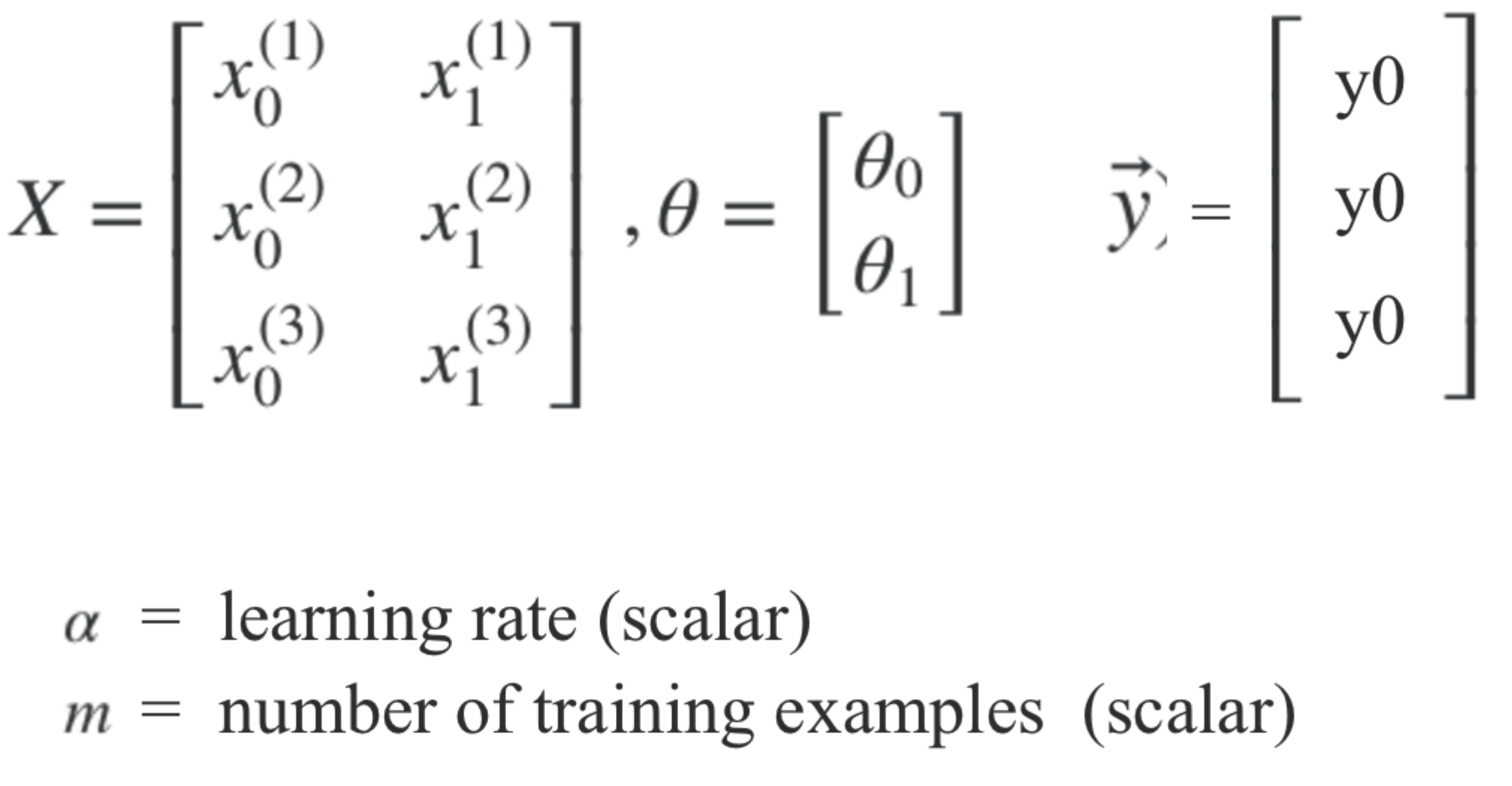
Now with multiple features, with multiple training examples, you can construct vectors of X and Theta like this.
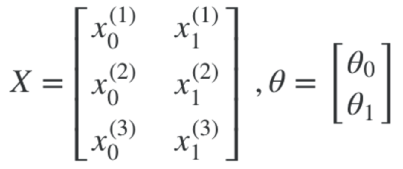
Note: Where the first row of the X matrix represents one training example
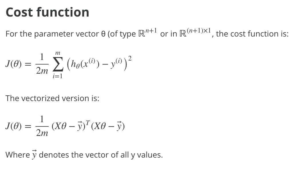
Cost function
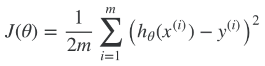
Recall that the cost function, for all training examples is this. (Also known as the "mean squared error")
We can replace h(x) now with the vectorised form in the previous list. This is the form for multiple features, and multiple training examples.
Vectorised Cost Function - Therefore, the vectorised version of the cost function now becomes this, where XTheta is the hypothesis
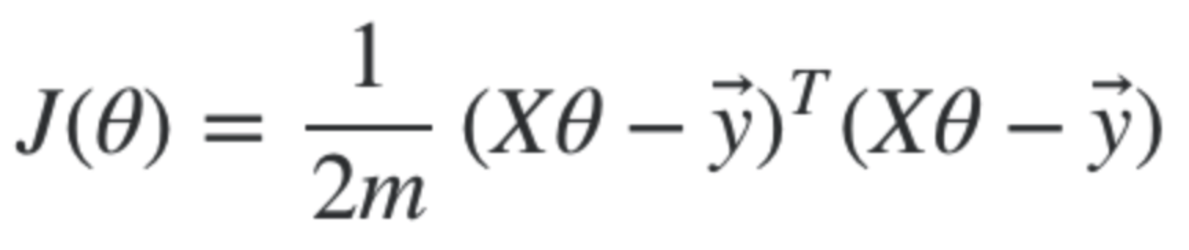
Remembering that X * Theta is the vectorised hypothesis
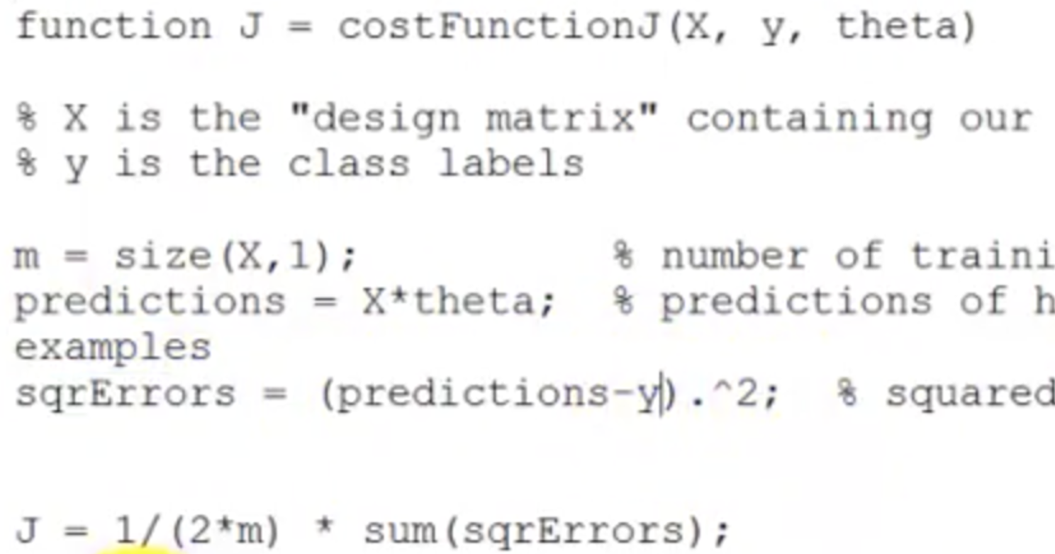
Code. Vectorised
Now, because we have arranged theta, X and y as matrices, we can translate the hypothesis into vectorised code
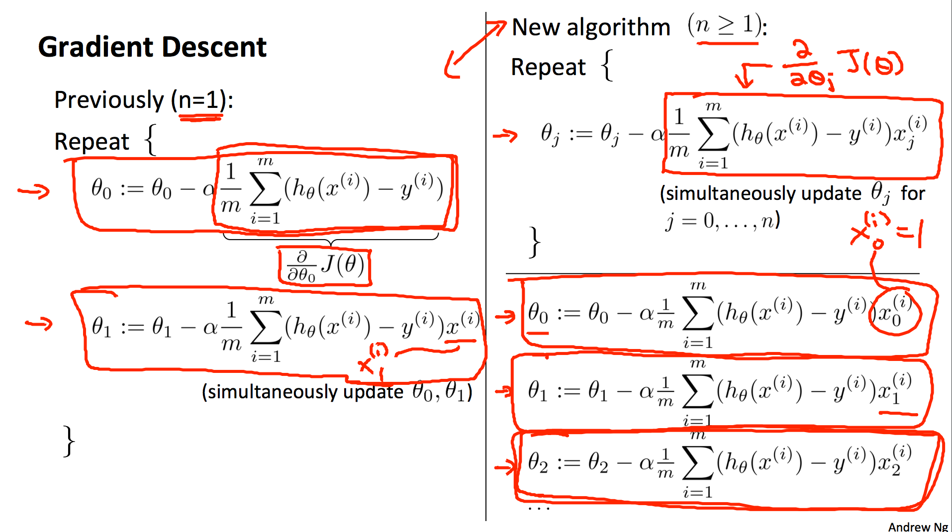
Multivariate Gradient Descent
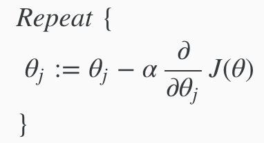
The general form for gradient decent
Gradient Descent is a process that lets you "descend" down the cost function in order to find the minimum/optimal theta values of the cost function
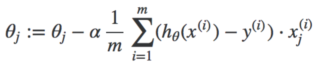
Gradient descent algorithm. Repeat this until it converges, where j = 0 to n number of features. Theta j, x j, and y are all matrices.
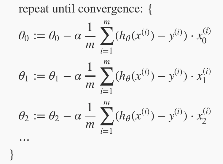
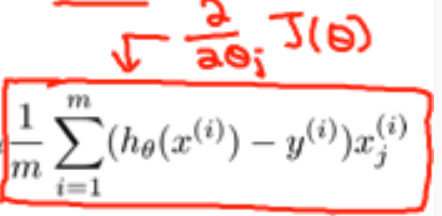
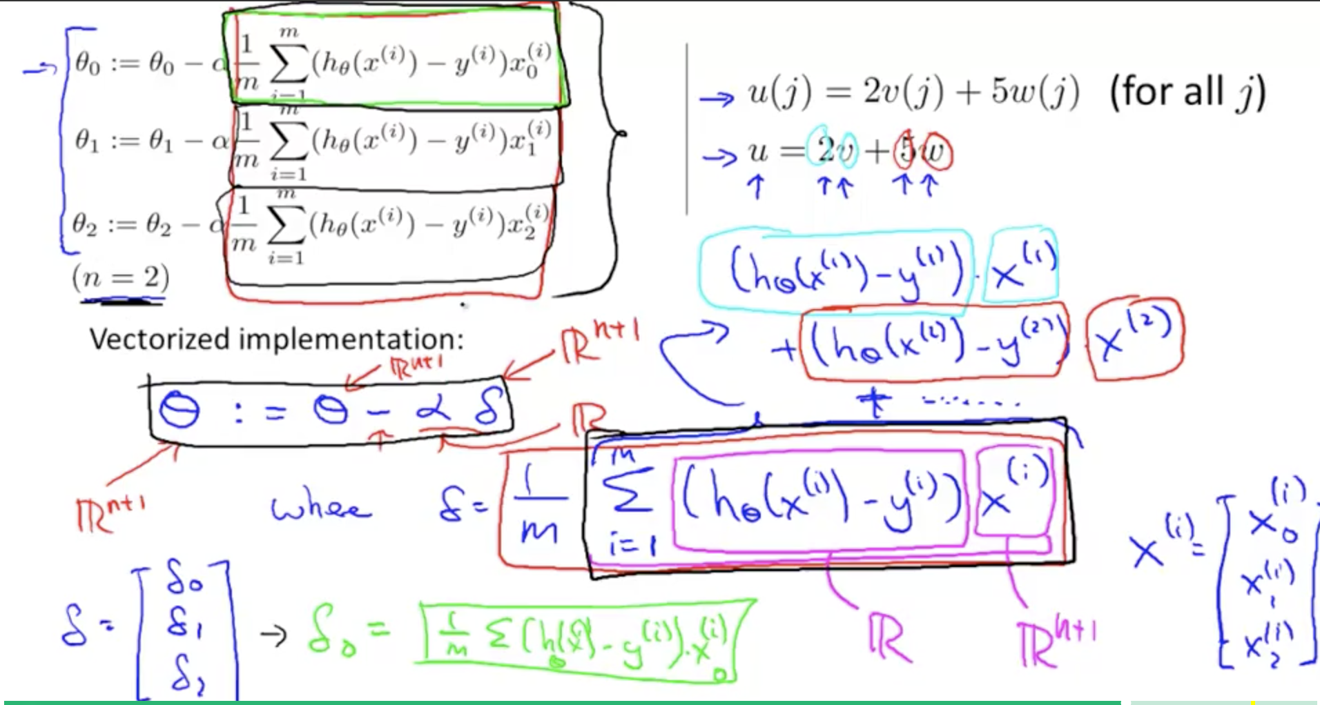
Breaking down the above, into it's seperate components for each Theta. Similar to univariate, but now generally we compute the descent for each ø in the cost function (remember that for each ø{j} you want to get the partial derivative with respect to j)


Additional Notes
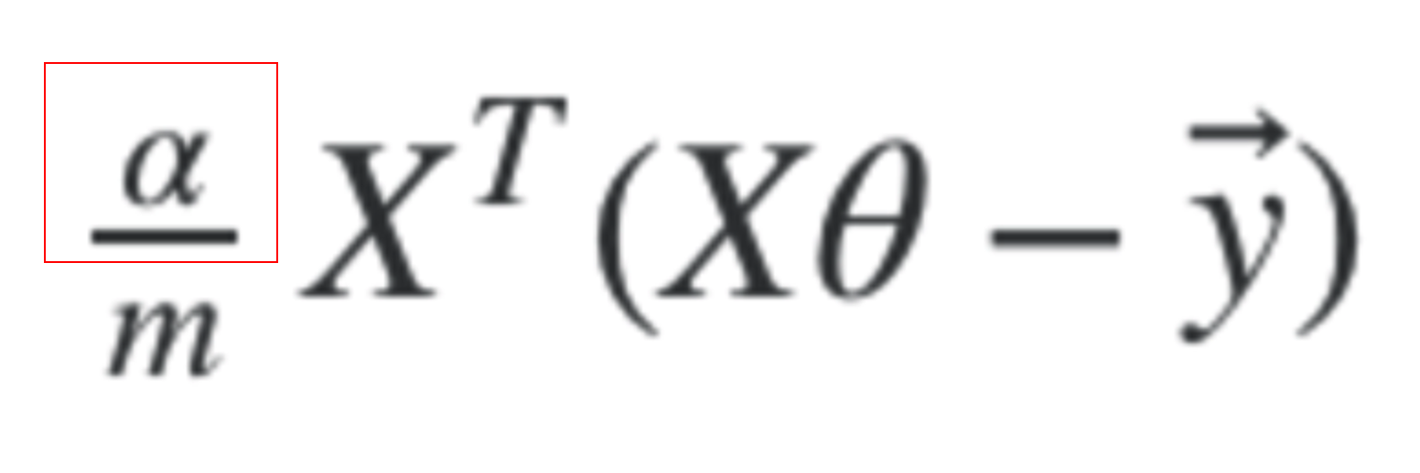
Remember also that this section of the function is the derivative of the J with respect to theta

Gradient Descent Vectorised
The vectorised form of Gradient Descent is this.
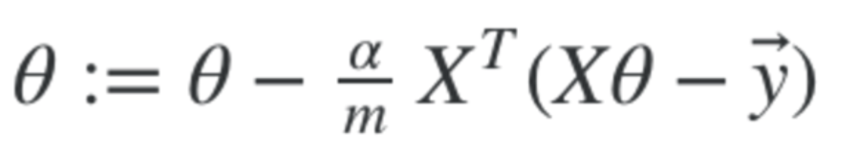
Where X, theta and y are all matrices. Alpha is the learning rate and is a scalar. And m is the number of training examples.
Additional Notes.
Gradient Descent - Vectorized!
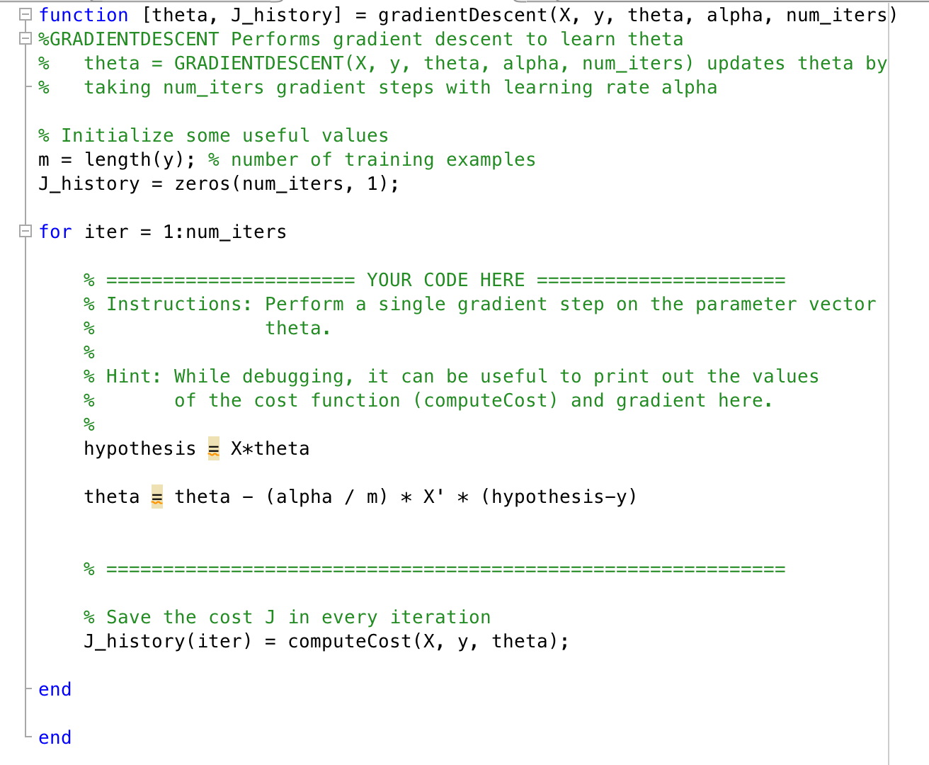
Code
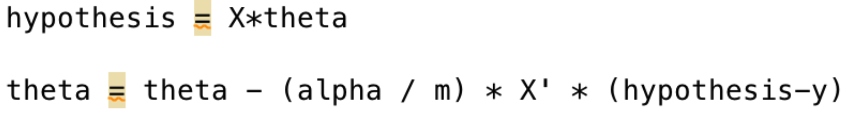
A single gradient descent step in Matlab code. We perform this for each gradient step iteration. X, hypothesis and theta are all matrices.
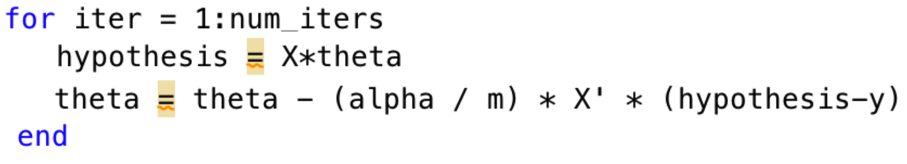
Full code example, with iteration loop
Learning Rate - alpha
The learning rate is a scalar value, alpha
You need to choose an appropriate value of the learning rate alpha to tune gradient descent, to make sure that convergence happens (ie stops decreasing by non-trivial amounts)
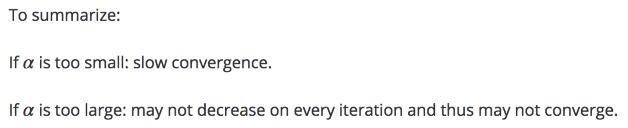
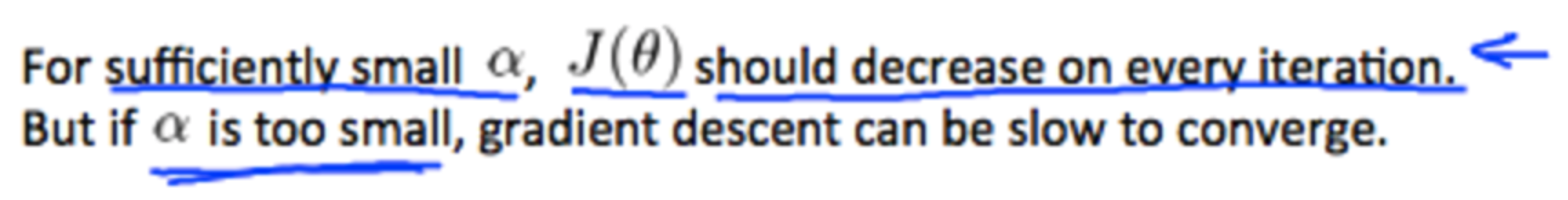
If you set the learning rate too small, convergence will be slow. If you set it too high, is may not converge at all
Additional Notes.
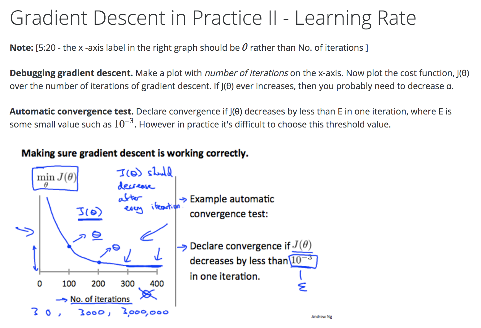
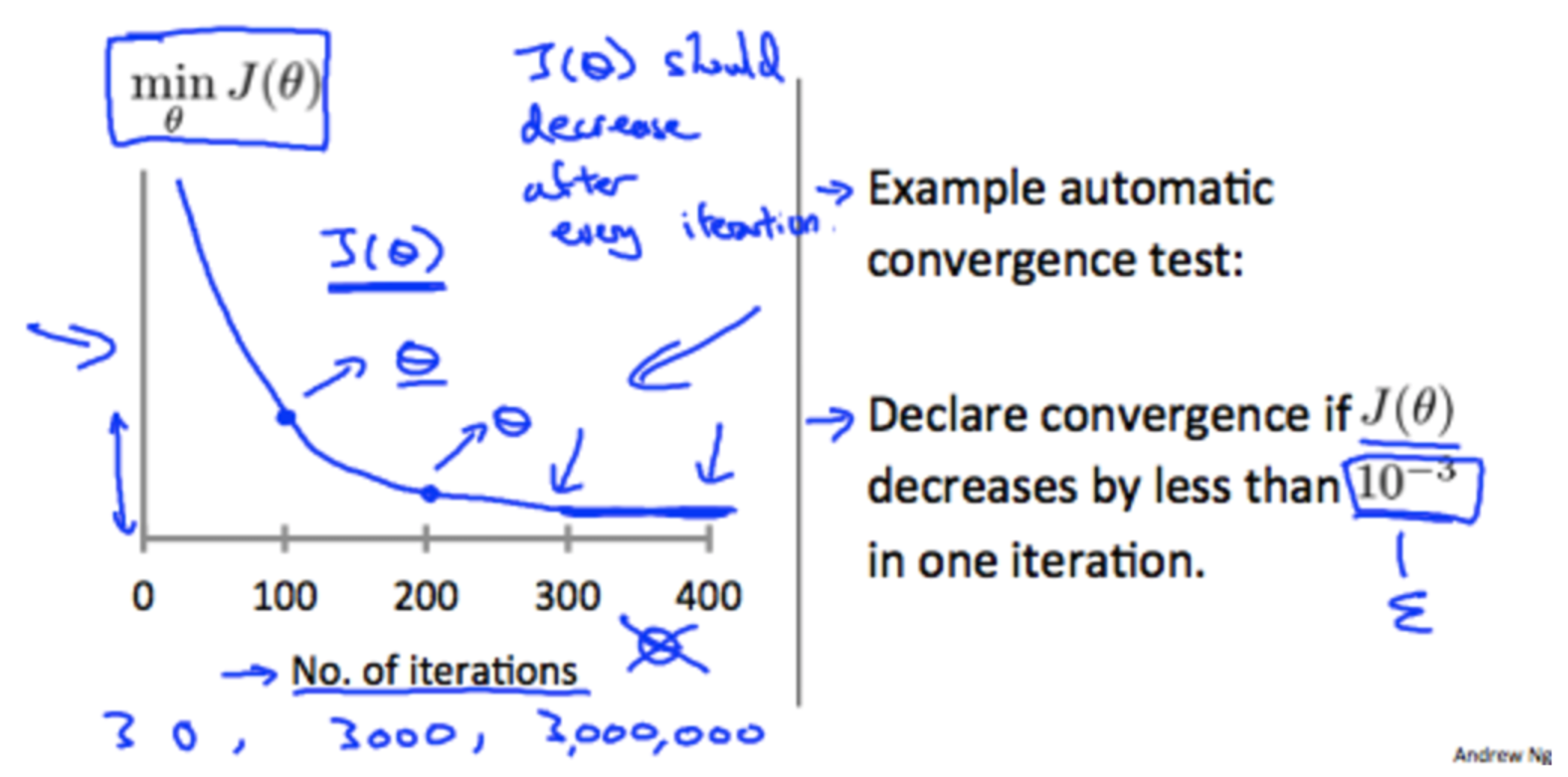
To make sure gradient descent is working, plot the cost J theta, against the number of iterations, and make sure it is decreasing. If it decreases by less than a sufficiently small value (say 10 to the -3) then we can declare that gradient descent has converged.
Summarising learning rate guidelines for alpha
Normal Equation with Octave
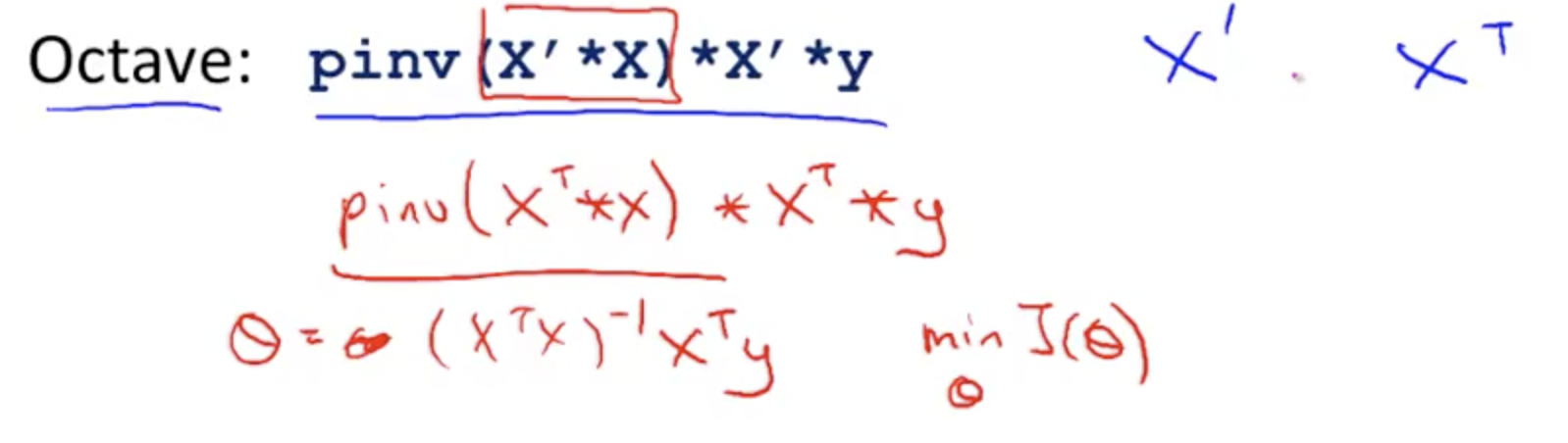
The equivalent in Octave of X(Transpose) is X' (Prime). So in Octave to compute ((X(Transpose)X)(inverse)) X(Transpose)Y - we can write pinv(X' X) X' * Y
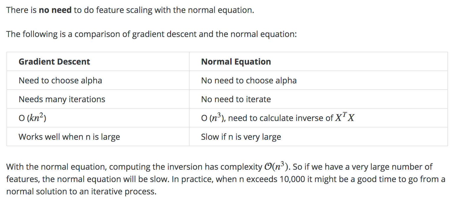
Gradient Descent vs Normal
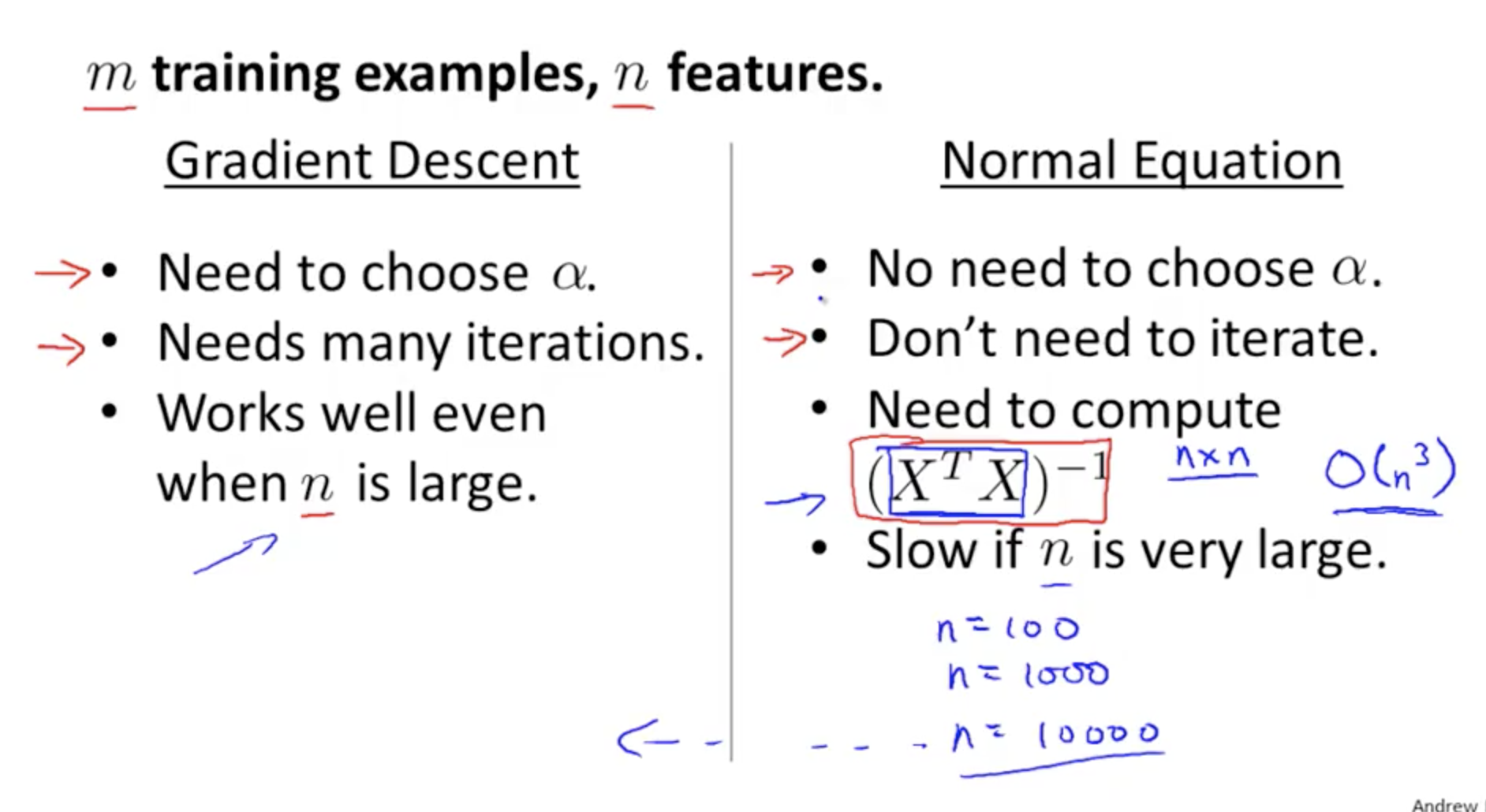
Summary
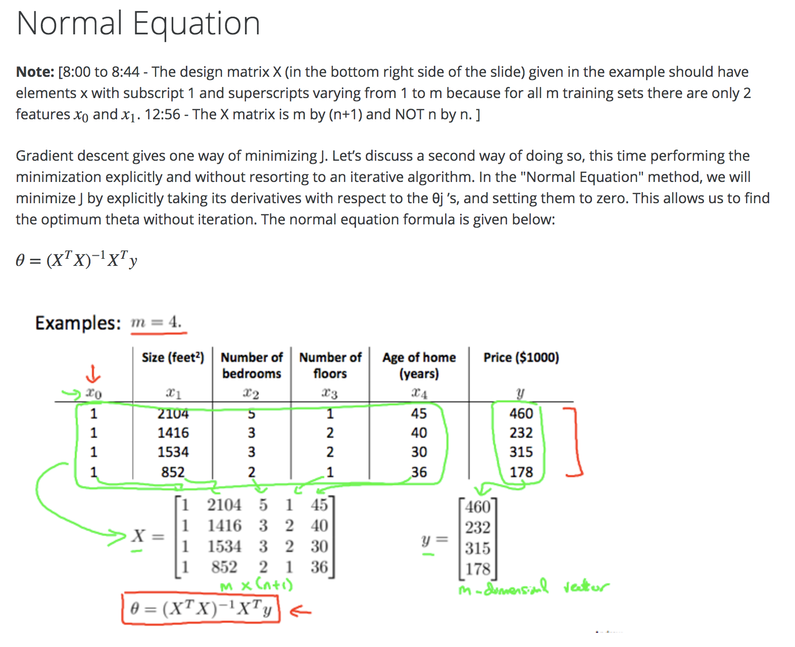
Normal Equation
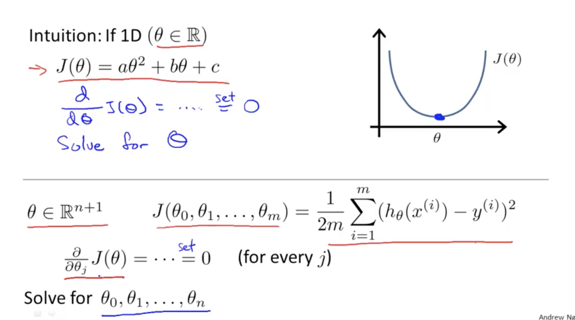
Normal equation, solves directly for the minimised cost function J
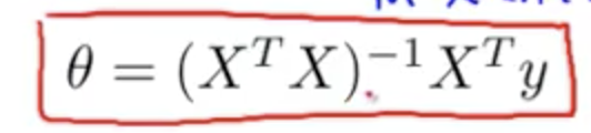
Basically set dx.J(ø) = 0 for every j
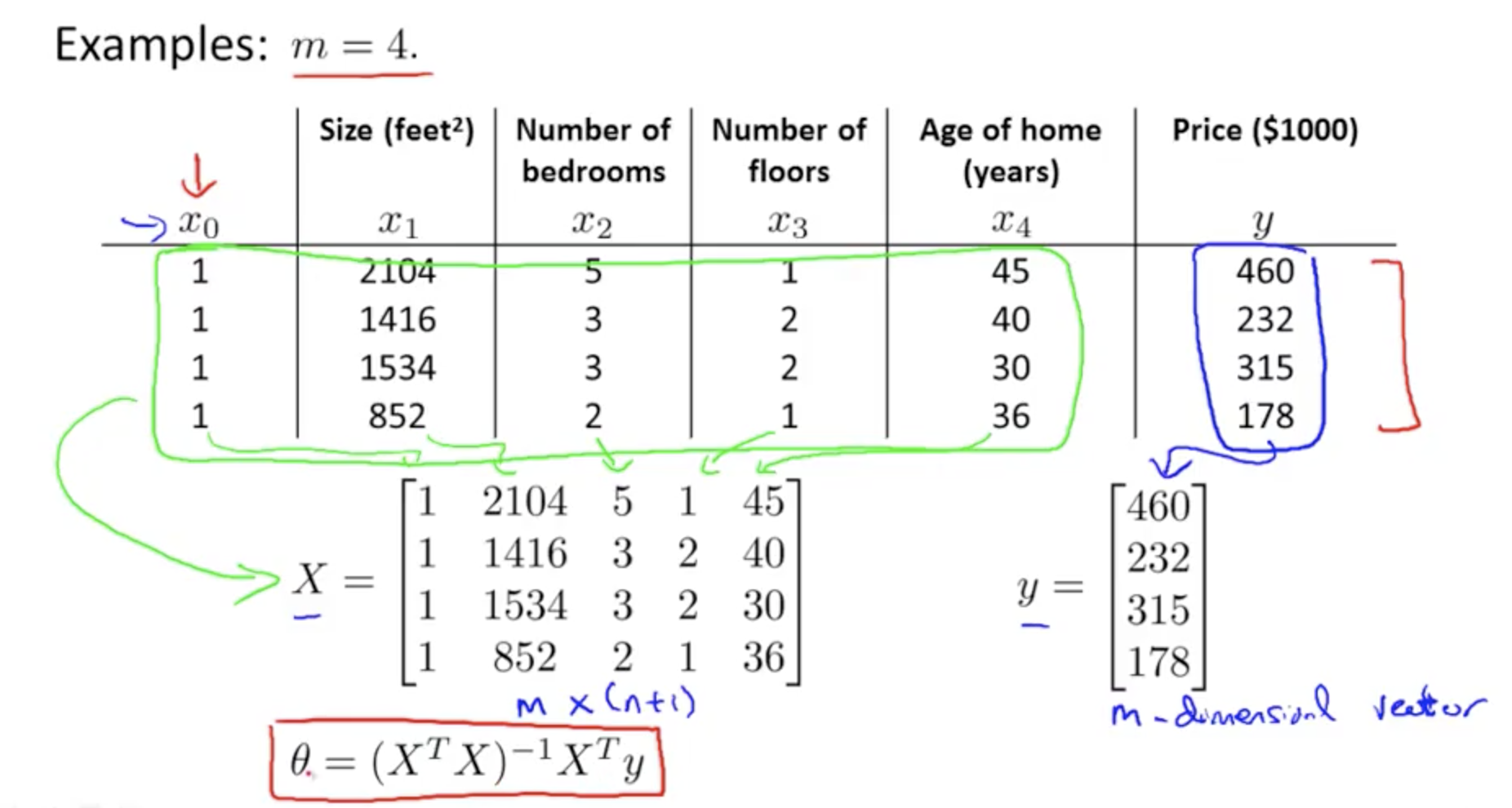
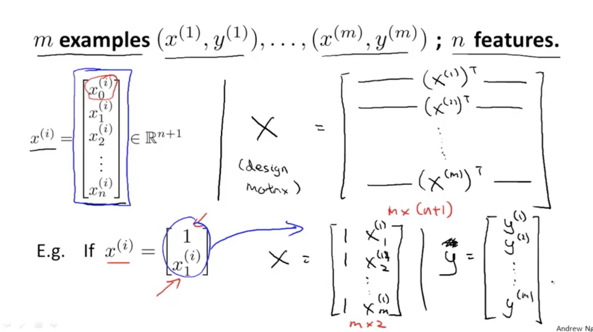
Example ...
If for one training example ...
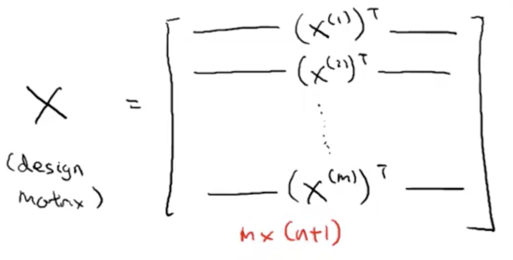
Matrix X - To calculate the design matrix X ...
Matrix Y - To calculate the matrix Y (its simply the vector of all results in the training example)
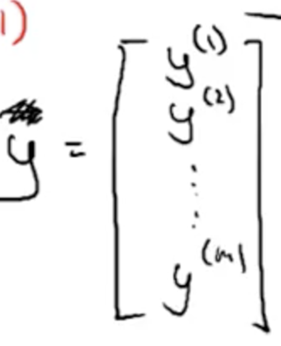
in summary, for X, and Y ....
X is the design Matric
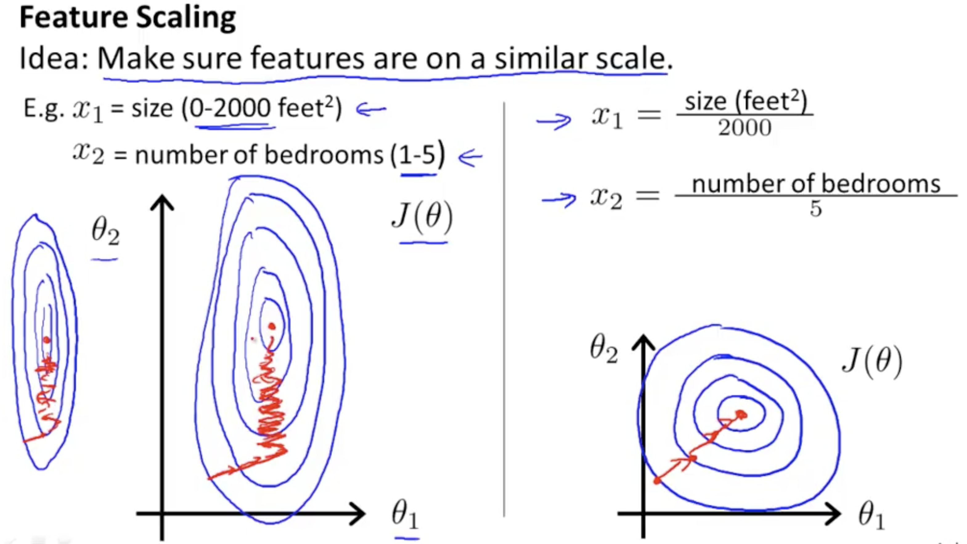
Feature Scaling
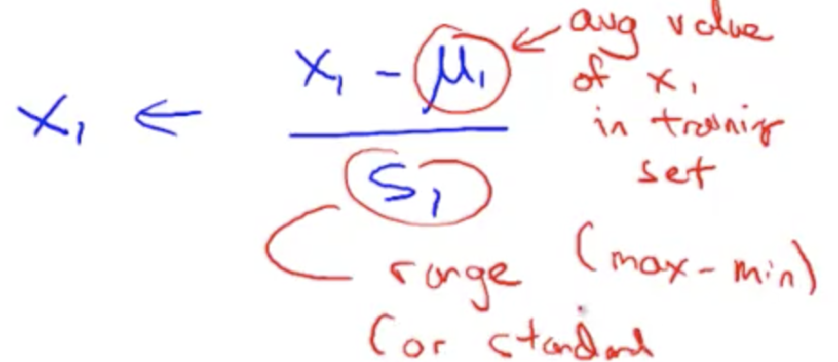
Diviiding by the max-min value should get x in approximately these values -1 < x < 1
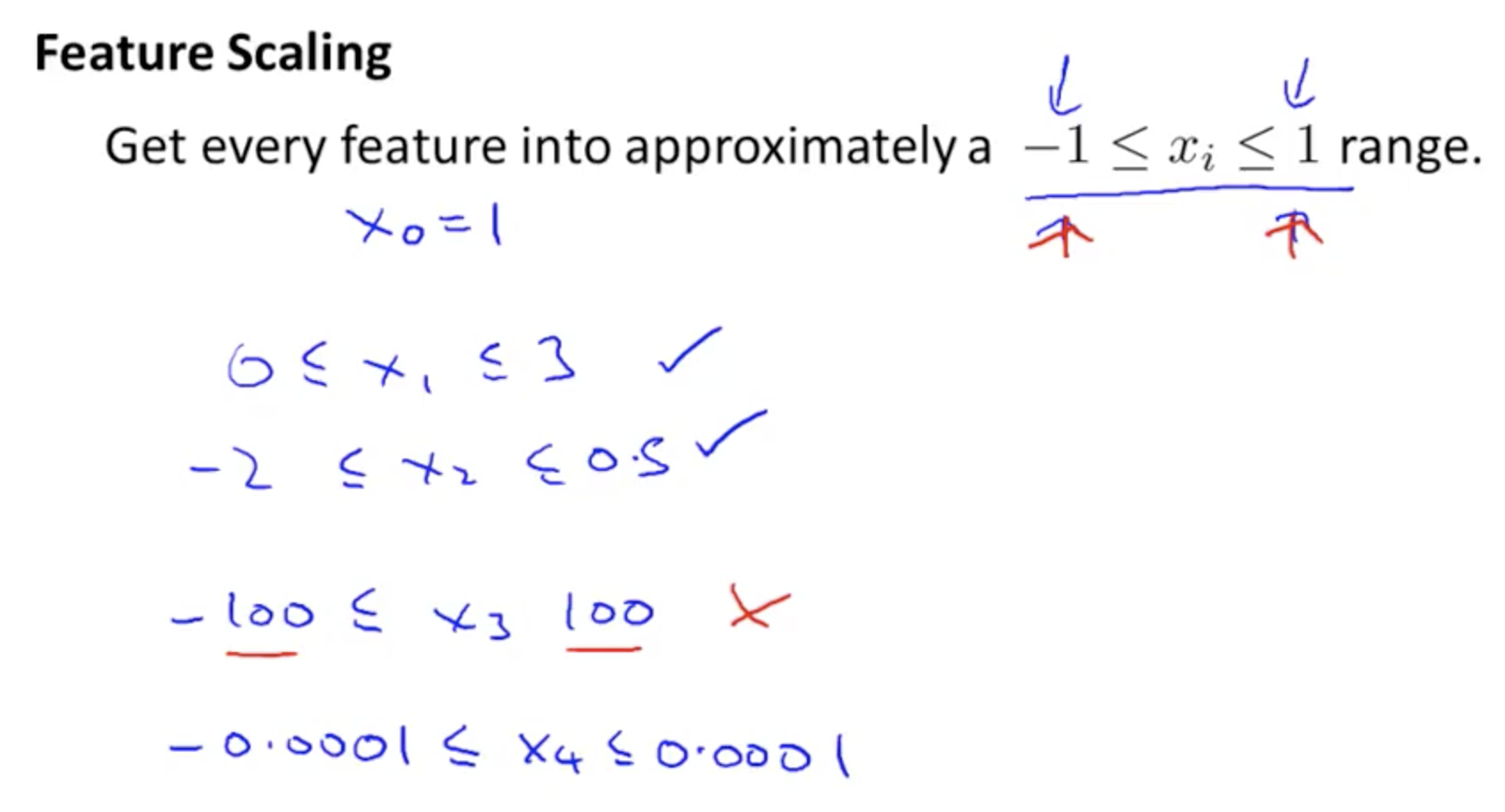
We use feature scaling so gradient descent uses less steps to exectue
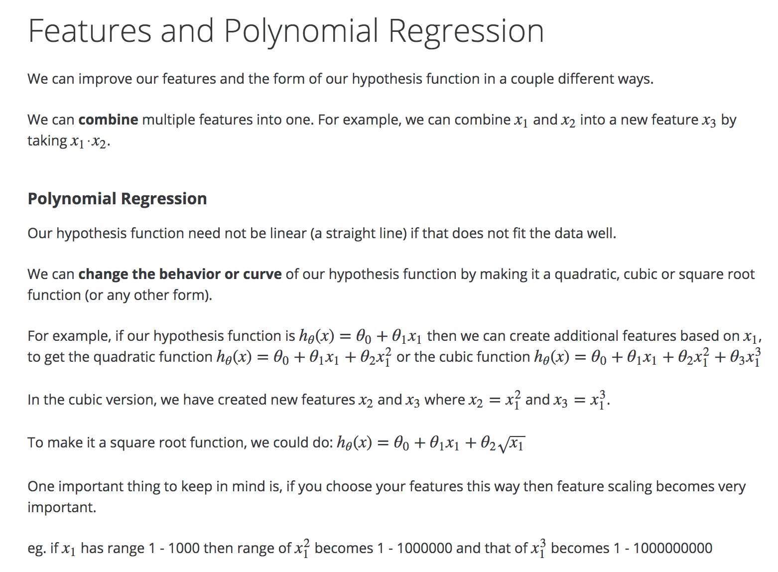
Features and Polynomial Regression
Polynomial Regression. If you choose your features in this way, then feature scaling becomes very important.
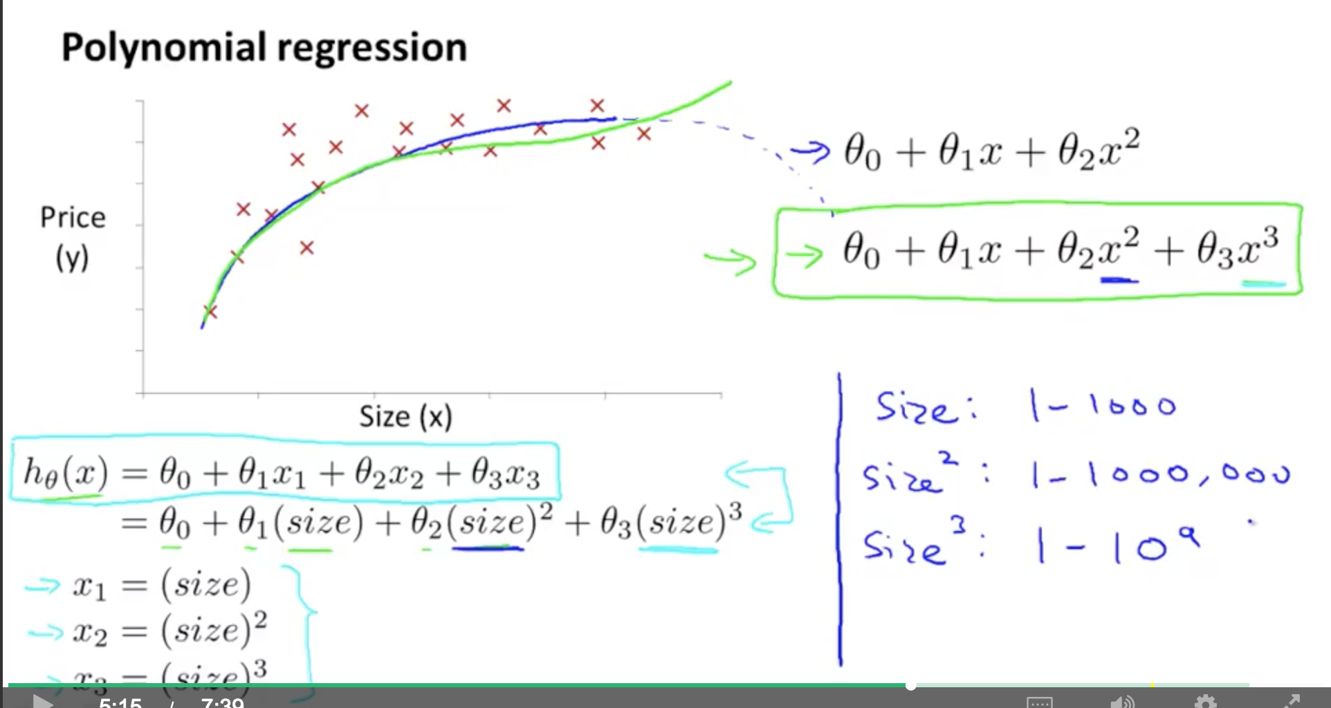
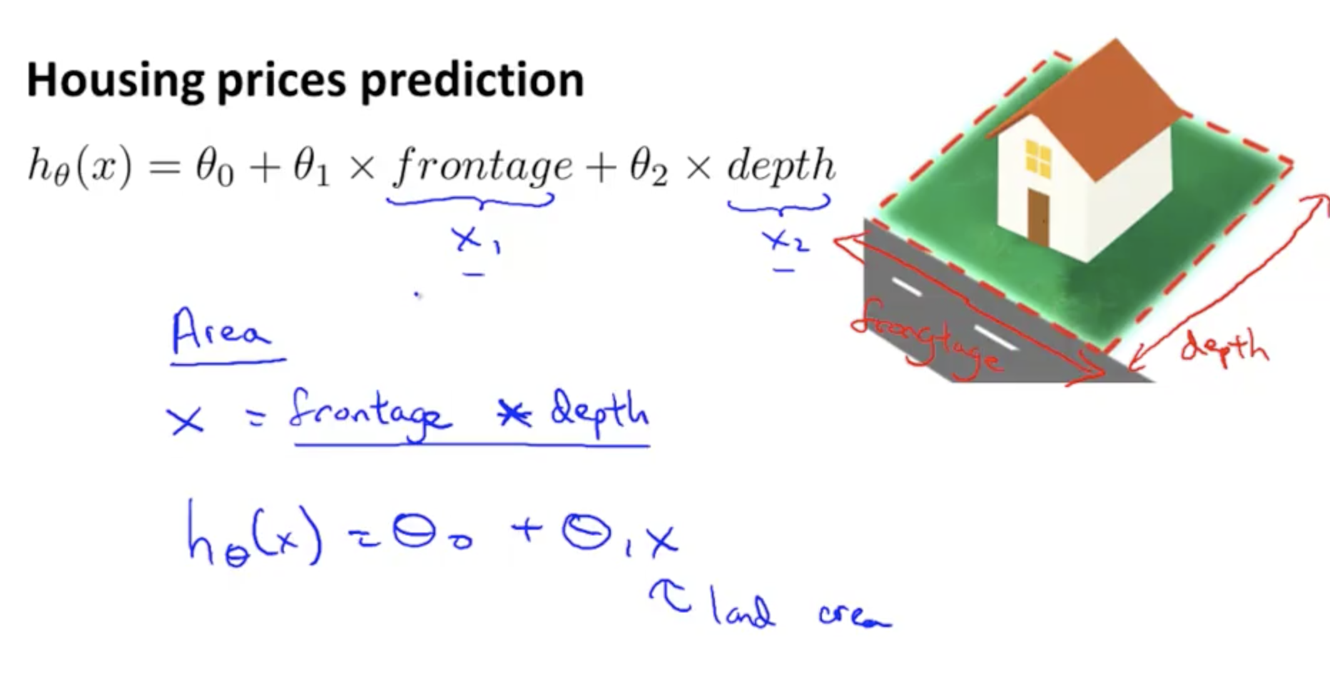
As an example, you can combine features to simplify a hypothesis expression
Summary:
Mean Normalization
Take (x - average of x) / max - min
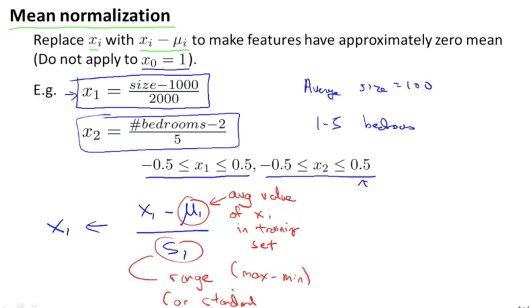
... in other words